This beginner-friendly course introduces data analysis using Python, covering fundamental libraries including NumPy for numerical computing, Pandas for data manipulation and analysis, and Matplotlib for visualization, enabling learners to perform exploratory data analysis on real-world datasets through hands-on practice and a final course project.
Python for Data Analysis: Numpy, Pandas & Visualization
Added:Deep Dive
Basic Python programming syntax, including variables, data types, loops, conditional statements, and custom functions.

Aprende a programar desde CERO en Python
85.6K
Python is an interpreted, imperative language designed for readability with minimalist syntax. Variables store values without explicit type declaration (weak typing), allowing type changes during runtime. Variable names can start with letters or underscores, contain numbers, but not start with numbers. Python is case-sensitive. The four primitive data types are integers, floats, strings (defined with quotes), and booleans (True/False). Type casting converts between types using int(), str(), and float() functions. Primitive types are assigned by value, while complex types are assigned by reference. Arithmetic operations (+, -, *, /, //, %) work on numbers, while strings use + for concatenation and * for repetition. Compound assignment operators (+=, -=, *=) combine operations with assignment. The print() function displays output and can accept multiple arguments. Python libraries provide pre-written functionality and are imported using import library, from library import function, or from library import *. The input() function pauses execution and stores user input as strings. Conditional statements (if, elif, else) control code execution based on conditions, with indentation defining code blocks. Logical operators (>, <, >=, <=, ==, !=) evaluate conditions and return True/False. Conditions combine using 'and' (both must be True) and 'or' (at least one must be True). For loops repeat code a known number of times using range() and iterate through sequences. While loops repeat while conditions remain True, requiring code changes to prevent infinite loops. Loop control statements include continue (skips current iteration) and break (exits loop immediately).
Click to watch →

02 - Basic Python (in Thai)
100
Python uses # for comments and = for variable assignment. Variables can be assigned in multiple ways: single assignment (a = apple), multiple assignment (a = apple, b = cherry), or list assignment (a = [apple, cherry]). Python distinguishes mutable (lists) from immutable (strings, numbers) data types. When assigning mutable objects to multiple variables, they share memory addresses, requiring copy() for independent copies. Conditional statements include if, if-else, and if-elif-else. Python uses indentation to define code blocks. Loop types include while (repeats while condition is True) and for (iterates through sequence items). The range() function generates sequences: range(start, stop, step) where stop is exclusive. Loop control statements include break (exits loop immediately) and continue (skips to next iteration). Functions are defined using def keyword: def function_name(parameters): followed by indented body. Functions can return values using return. Lambda functions are anonymous: lambda arguments: expression.
Click to watch →
【Python】(if,for,配列)基本文法必ず使う!たったこれだけで、10分でプログラムが書けるようになる!
3.1K
Python's core programming concepts include declaring variables with values using the '=' operator, using lists as arrays with square brackets, implementing loops with 'for' statements, and creating conditional logic with 'if', 'elif', and 'else' statements; Python's distinctive features include indentation-based code blocks (4 spaces), no explicit type declarations, and a procedural programming paradigm that makes code concise and readable.
Click to watch →

Aprende Python Curso para principiantes | Pt 1 Primeros Pasos
799
Variables are memory spaces for storing data, declared with name = value syntax. Python has four basic types: integers (whole numbers), floats (decimals), strings (text in quotes), and booleans (True/False). The print() function displays values in the console. String operations include concatenation (+) and repetition (*). Arithmetic operators include +, -, *, /, // (integer division), % (modulus), and ** (exponentiation). Comparison operators (==, !=, >, <, >=, <=) evaluate relationships and return True/False. Logical operators (and, or, not) combine boolean values. Compound assignment operators (+=, -=, *=, /=, //=, %=, **) combine operations with assignment. Conditional structures enable decision-making: 'if' executes when True, 'elif' checks additional conditions, 'else' executes when all previous failed. Python uses indentation (4 spaces) to define code blocks. For loops repeat code a specified number of times using 'for i in range(n)', where range() generates sequences. While loops repeat as long as a condition remains True, requiring manual variable updates to prevent infinite loops. Break exits loops immediately, while continue skips to the next iteration.
Click to watch →

PYCON US 2013 - Learn Python Through Public Data Hacking
4K
Python programs consist of statements separated by newlines, executed top to bottom. Comments start with a pound sign (#). Variables are assigned using '=' without declaring types - the type comes from the assigned value. Basic data types include integers (whole numbers), floating-point numbers (with decimal points), and strings (enclosed in single or double quotes). Strings have operations like len(), + (concatenation), upper(), starts_with(), and replace().
Click to watch →
Deep Dive
Fundamental mathematical and statistical concepts, such as mean, median, standard deviation, and basic probability.

Mean, median, Probability
102
This video covers three essential statistical concepts. First, calculating the mean involves dividing the total sum of numbers by the count of numbers; when adding a new number, recalculate the total and divide by the new count. Second, finding the median requires arranging numbers in order; for even-sized data sets, average the two middle numbers. Third, the probability of either event A or B occurring uses the formula P(A or B) = P(A) + P(B) - P(A and B), which accounts for overlapping events to avoid double-counting. These concepts form the foundation of descriptive statistics and probability theory.
Click to watch →
Bias And Variance In Statistics | Bias And Variance Explained | Learn Statistics | Simplilearn
3.7K
Statistics is the science of collecting, analyzing, and interpreting empirical data. Three key measures of central tendency are: (1) Mean (average) calculated by summing all values and dividing by count; (2) Median, the middle value when data is ordered, less affected by outliers; (3) Mode, the most frequently occurring value. Standard deviation measures data dispersion relative to the mean, calculated as the square root of variance. In a normal distribution (bell curve), one standard deviation covers ~68% of data, two cover ~95%, and three cover ~99.7%. Standard deviation is expressed in original units, making it more interpretable than variance.
Click to watch →
Statistics: Standard deviation | Descriptive statistics | Probability and Statistics | Khan Academy
2.3M
This segment covers three core statistical concepts essential for data analysis. The mean (μ for populations, x̄ for samples) represents the central tendency, calculated as the sum of data points divided by their count. Variance (σ² for populations, s² for samples) measures dispersion—the average squared distance from the mean. For populations, divide by N; for unbiased sample estimates, divide by (n-1). Standard deviation (σ or s) is the square root of variance, returning to original measurement units for better interpretability. These measures together describe both the central location and spread of a dataset.
Click to watch →

Class - 7, Bharti Bhavan, Sugam Ganit, , Vividh - 7 , Q.no - 1 to 3 ii
12.7K
This comprehensive lesson covers three fundamental statistical concepts. Mean (average) is calculated as sum of all values divided by count of values. The formula can be rearranged to find sum (mean × count), count (sum ÷ mean), or unknown values. Median is the middle value when data is ordered—middle value for odd counts, average of two middle values for even counts. Probability measures likelihood as favorable outcomes divided by total possible outcomes. These concepts form the foundation of descriptive statistics and probability theory.
Click to watch →
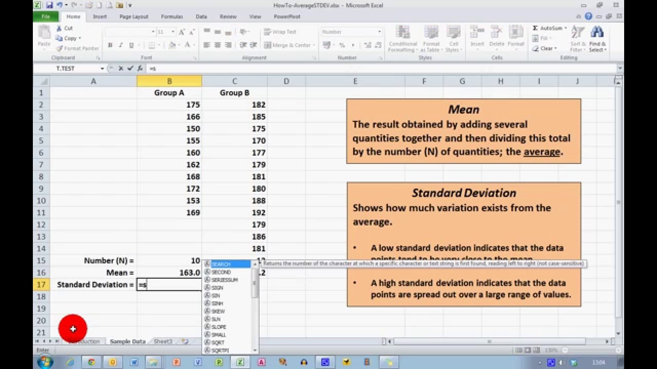
How To... Calculate Mean and Standard Deviation in Excel 2010
955.8K
The mean represents the average value of a dataset, calculated by summing all values and dividing by the number of values. Standard deviation measures how much data varies from the mean—low values indicate data points cluster closely around the average, while high values show wide data spread. These two statistics form the foundation for comparing datasets, allowing researchers to identify central tendencies and variability patterns within their data.
Click to watch →
Deep Dive
Familiarity with tabular data structures, such as spreadsheets, and common file formats like CSV and Excel.

CS 220 Data Programming I: Lecture 14 Tabular Data and CSV Files
1.2K
This segment covers working with tabular data and CSV files. Tabular data organizes information in rows and columns, similar to spreadsheets. CSV (Comma Separated Values) is a standard text format for storing tabular data with key characteristics: one sheet per file, all data stored as strings (numbers must be converted), no formatting options, and no formulas. Unlike Excel's binary format, CSV files are plain text and easily readable by humans and programs. The Python csv module provides tools for reading CSV files using csv.reader(), which returns an iterator yielding rows as lists. The data is stored as a list of lists, where rows[0][0] accesses the first element of the first row. This structure allows efficient access to specific data points using nested indexing.
Click to watch →

Reading csv, tsv, and xlsx files with Python
7.6K
This video demonstrates how to read data from three common spreadsheet file formats (CSV, TSV, and XLSX) into two Python data structures: DataMatrix objects using the data_matrix library and Pandas DataFrames using the pandas library. The key insight is that different file formats can be unified into the same data structure, with the main consideration being the correct specification of delimiters (comma for CSV, tab for TSV) when reading tabular data.
Click to watch →

Excel 2016 Tutorial: A Comprehensive Guide on Excel for Anyone
766.7K
CSV (Comma-Separated Values) files store tabular data with commas separating fields. To import a CSV file, go to File > Open, browse to the file, and Excel will detect it as a text-delimited file. In the import wizard, confirm the file has headers (first row contains labels), specify comma as the delimiter, and click Finish. Imported data appears in a new worksheet ready for analysis.
Click to watch →

Python. Работа с файлами csv
7.2K
CSV (Comma-Separated Values) is a text-based file format for storing tabular data where values are separated by commas. TSV (Tab-Separated Values) uses tabs instead. Both formats are universal and supported by spreadsheet applications like Excel. To import CSV files in Excel, use Data > Get External Data > From Text, then configure delimiters and specify header rows. Excel supports various delimiters and provides preview functionality. After import, you can configure column formats for each field. Converting Excel tables to CSV involves using Save As with CSV format and specifying custom delimiters.
Click to watch →
![สอน Python & Pandas | สำหรับจัดการและวิเคราะห์ข้อมูล [FULL COURSE]](https://i.ytimg.com/vi/SPdwqEPZ_EE/hqdefault.jpg)
สอน Python & Pandas | สำหรับจัดการและวิเคราะห์ข้อมูล [FULL COURSE]
91.8K
To read a CSV file into a DataFrame, use 'pd.read_csv(filename, encoding='utf-8')'. The 'filename' parameter specifies the path to the CSV file. The 'encoding' parameter specifies the character encoding (default is 'utf-8', but some files may use different encodings). To read only specific columns from a CSV file, use 'pd.read_csv(filename, usecols=[column1, column2, ...])'. The 'usecols' parameter is a list of column names to include in the resulting DataFrame. To read an Excel file into a DataFrame, first install the 'openpyxl' library using 'pip install openpyxl'. Then use 'pd.read_excel(filename, sheet_name='sheet1', encoding='utf-8')'. The 'filename' parameter specifies the Excel file path. The 'sheet_name' parameter specifies which sheet to read (default is the first sheet). To read a specific sheet from an Excel file, use 'pd.read_excel(filename, sheet_name='sheet_name')'. The 'sheet_name' parameter can be a string (sheet name), an integer (sheet number), or a list of sheet names.
Click to watch →
Deep Dive
Basic usage of a Python execution environment, preferably Jupyter Notebooks, Google Colab, or VS Code.

Proyecto 4.0 Segunda edición - Python y la Automatización Industrial - IngeLearn
10.1K
Google Colab is an online Jupyter notebook environment for executing Python code in the browser. To use it: connect to a server (button in top-right corner), then click play on code cells. The print() function outputs text to the console. A simple 'Hello World' program requires just one line: print('Hola mundo'). This demonstrates Python's simplicity compared to compiled languages like C++. The Colab environment includes markdown cells for explanations and code cells for executable Python, making it excellent for learning and collaborative development.
Click to watch →

Full Python Live Course For Beginners 🔥 Session 1 🔥 Python Tutorials 🔥 Learn Python for FREE
20.5K
The 15-day Python course covers: Introduction to Python, Variables and Data Types, Operators, Strings, IO Modules, Classes and Objects, Inheritance, Exception Handling, and Bonus topics including APIs and HTTP handling. A capstone project will be included. For beginners, Google Colab (Jupyter Notebook) is recommended as it requires no installation and allows immediate coding. Anaconda with Jupyter Notebook is another option. Local IDEs like PyCharm, VS Code, or Atom can be used later. Jupyter Notebook has two types of cells: Code cells (for writing Python code) and Text cells (for writing notes and comments). Code cells execute Python code and display output. Text cells allow formatting with bold, italic, and other styles. The print() function displays strings enclosed in double or single quotes. Code execution can be done by clicking the play button or pressing Shift+Enter.
Click to watch →

Let's Get You That $250,000 Job! | Python Tutorial | PART 1 | Martin Shkreli
37.2K
Anaconda Navigator launches VS Code pointing to Anaconda's Python version. Git is optional for version control and sharing projects. When first opening VS Code, you may be prompted to make decisions, then the interface appears with options for extensions. To select your Python interpreter, use View > Command Palette (Ctrl+Shift+P) > Select Interpreter. To run Python, click View > Terminal (Ctrl+`) and type 'python' to enter the REPL (Read-Evaluate-Print Loop) where you can type code and see immediate results. Jupyter Notebook is web-based, supporting Python, Julia, and R. The name 'Jupyter' comes from these three languages. The 'Notebook' part refers to the paper notebook structure where code is placed. Cells can contain code or text/pictures. To write code, select 'Code' from the toolbar dropdown. Unlike the Python interpreter, code must be run by clicking the Run button. The file extension is .ipynb (IPython Notebook). In VS Code, use Ctrl+Enter or Alt+Enter to run code in Jupyter. To check Python version, type 'python --version' in the terminal. The Python interpreter prompt is called the REPL. Typing something undefined results in an error message, but nothing is broken. To get help, type 'help()' with parentheses, which shows keywords and tutorials. Python has a small number of keywords that can be memorized. To exit help mode, press Enter repeatedly, Q, or Ctrl+Z. Creating apps requires a VS Code development environment, which is the Python interpreter plus extensions. You can save workspaces using File > Save Workspace As.
Click to watch →

Atelier de programare Python pentru începători
4.6K
Python development environments include Jupyter Notebook, Visual Studio Code, and PyCharm. Google Colab provides a free online Python environment accessible through Google. To use Colab, search for 'Google Colab', click 'New Notebook', and press 'Connect'. Settings can be adjusted to enable line numbers for better code navigation.
Click to watch →

DAY-5: Python Tools Explained: Jupyter Notebook, Google Colab & VS Code | Complete AI Journey
265
This lecture explains three essential Python development tools: Jupyter Notebook (.ipynb files) for iterative, cell-by-cell code execution ideal for data science and AI work; Google Colab as a cloud-based alternative requiring no local installation; and Visual Studio Code (.py files) for traditional Python script development. The instructor demonstrates how to set up each tool, create and run code, and manage files, while emphasizing that Python is case-sensitive and that tool selection depends on the development context—Jupyter Notebook for exploratory data analysis and Google Colab for collaborative cloud-based work.
Click to watch →
Prerequisite Knowledge
- Concept 01Basic Python programming syntax, including variables, data types, loops, conditional statements, and custom functions.
- Concept 02Fundamental mathematical and statistical concepts, such as mean, median, standard deviation, and basic probability.
- Concept 03Familiarity with tabular data structures, such as spreadsheets, and common file formats like CSV and Excel.
- Concept 04Basic usage of a Python execution environment, preferably Jupyter Notebooks, Google Colab, or VS Code.
Subsequent Learning
- Step 01Introduction to Machine Learning concepts and predictive modeling using the Scikit-Learn library.
- Step 02Advanced data visualization and interactive dashboard creation using libraries like Plotly, Seaborn, and Streamlit.
- Step 03Database integration, including querying databases using SQL and loading results directly into Pandas DataFrames.
- Step 04Feature engineering and advanced data preprocessing techniques for handling missing values, outliers, and categorical encoding.
- Step 05Scaling to Big Data using distributed computing frameworks such as PySpark or Dask.
Course Overview
Target Audience
Learning Outcomes
Practice & Project
Prerequisites
Course Overview
0:00Playing Section
- 1
Practical, beginner-friendly data analysis course.
- 2
Live online with verified certificate option.
The R Ecosystem and Tidyverse for Data Science
While Python is a general-purpose language adapted for data science, R was built from the ground up specifically for statistical computing and visualization. For students learning data analysis, the R ecosystem—particularly the "Tidyverse" (which includes dplyr and ggplot2)—offers a highly cohesive, intuitive, and mathematically rigorous alternative to the NumPy/Pandas/Matplotlib stack. Unlike Pandas, which is often criticized for its inconsistent syntax and heavy memory overhead, the Tidyverse is designed with a unified philosophy that makes data manipulation and exploratory data analysis (EDA) highly readable and expressive. Furthermore, R remains the gold standard in academic research, bioinformatics, and advanced statistics due to its superior out-of-the-box statistical modeling capabilities. Learning R provides a distinct, data-first paradigm that contrasts with Python's software-engineering-first approach, broadening a student's perspective on how to interact with data.
Deep Dive
Introduction to Machine Learning concepts and predictive modeling using the Scikit-Learn library.

Sebastian Raschka | Learning scikit learn - An Introduction to Machine Learning in Python
23.9K
This tutorial introduces machine learning fundamentals using scikit-learn, covering supervised learning (regression and classification) and unsupervised learning (clustering), with practical examples including linear regression for predicting brain weight from head size and logistic regression/KNN classification on the Iris dataset, emphasizing proper data splitting, model evaluation, and preprocessing techniques like feature scaling and label encoding.
Click to watch →

Jake VanderPlas: Machine Learning with Scikit Learn
45.8K
Machine learning involves training algorithms to make predictions from data, with scikit-learn providing a unified API for common tasks like classification (predicting discrete labels) and regression (predicting continuous values). Data must be structured as a 2D matrix where rows represent samples and columns represent features, with labels stored separately. The scikit-learn estimator pattern follows a consistent workflow: import a model class, instantiate it with hyperparameters, fit it to training data, and use predict() or predict_proba() on new data. Key supervised learning algorithms include k-nearest neighbors, support vector machines (which maximize margins between classes and use kernel methods for nonlinear boundaries), and random forests (ensembles of decision trees that reduce overfitting through averaging). Model validation and hyperparameter tuning are essential for preventing overfitting and selecting optimal models.
Click to watch →

Primeiros passos com Scikit-Learn | Machine Learning #04
53.2K
Scikit-learn is a Python package for machine learning that enables simple and efficient data analysis and predictions. Built on top of NumPy, SciPy, and Matplotlib, it supports classification, regression, clustering, dimensionality reduction, model selection, and preprocessing. The package provides built-in toy datasets like Iris (150 samples of 3 species with 4 features) and digits for learning. Documentation follows a consistent tutorial format with executable code examples. The mathematical notation X for features and y for target reflects the function concept y = f(x), where algorithms find the mapping from inputs to outputs.
Click to watch →
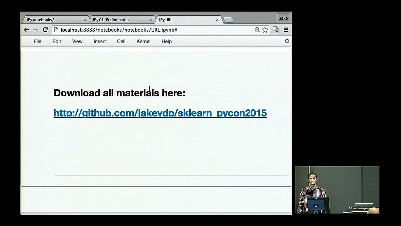
Jake VanderPlas - Machine Learning with Scikit-Learn (I) - PyCon 2015
62.1K
This tutorial by Jake VanderPlas provides an introduction to core machine learning concepts and the Scikit-Learn package. It covers the Scikit-Learn API and demonstrates how to use it to explore basic categories of machine learning problems. The session includes practical instruction on feature selection and model validation, key components in building effective machine learning workflows. Participants are guided through applying these tools to real-world datasets, emphasizing hands-on experience with the library. The tutorial is structured to help learners understand how to interface with Scikit-Learn for supervised and unsupervised learning tasks, though specific algorithms are not listed. The focus is on foundational usage patterns, data preparation, and evaluating model performance using the library’s built-in methods. No advanced mathematical theory or implementation details are described. The goal is to equip attendees with practical skills to begin using Scikit-Learn for common machine learning applications. Slides and code examples are made available online for reference, supporting the tutorial’s applied learning approach.
Click to watch →
Apprentissage statistique et analyse prédictive en Python avec scikit-learn - Alexandre GRAMFORT
33.2K
scikit-learn is a Python library for machine learning that provides tools for supervised learning (classification, regression), unsupervised learning (clustering, dimensionality reduction), and model evaluation, enabling practitioners to build predictive models by training algorithms on labeled or unlabeled data to discover patterns and make predictions.
Click to watch →
Deep Dive
Advanced data visualization and interactive dashboard creation using libraries like Plotly, Seaborn, and Streamlit.

Streamlit - Building Financial Dashboards with Python
170.5K
This section demonstrates building interactive charts using Plotly and Streamlit. The process involves: (1) importing plotly.graph_objects as go, (2) creating a go.Figure() and adding go.Candlestick() data with date, open, high, low, close values, (3) reading price data from a database using pandas.read_sql(), and (4) displaying the chart using st.plotly_chart(). The dashboard allows users to type in stock symbols and view interactive candlestick charts with pan and zoom functionality.
Click to watch →
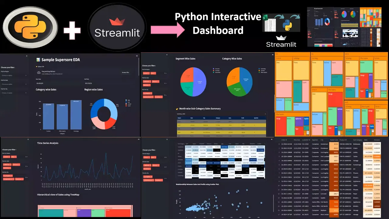
Python Interactive Dashboard Development using Streamlit and Plotly
266.8K
This video tutorial demonstrates how to build an interactive Python dashboard using Streamlit and Plotly libraries, covering essential concepts including data uploading, date filtering, multi-select sidebar filters, dynamic chart generation (bar charts, pie charts, time series analysis, scatter plots, and treemaps), and data downloading functionality. The instructor walks through creating a complete sales analytics dashboard from scratch using the Superstore dataset, showing how to implement responsive layouts, apply CSS styling, and create live-filtered visualizations that update automatically based on user selections.
Click to watch →

My Workflow for Building any Streamlit Dashboard Project
161.2K
Plotly Express provides a high-level API for creating interactive visualizations in Streamlit that closely resembles the syntax of pandas' plotting methods. It simplifies the creation of common chart types like line charts, bar charts, and scatter plots. The API automatically generates plotly figures with reasonable defaults, and additional customization options like titles, markers, and text annotations can be added through method arguments.
Click to watch →

Curso de Streamlit: Desarrolla Aplicaciones Web con Python Fácilmente (Parte 2)
6.4K
Plotly Express enables interactive data visualization in Streamlit applications. The workflow involves: (1) installing plotly library via pip, (2) reading CSV data using pandas pd.read_csv() into DataFrames, (3) aggregating data using groupby() for categorical analysis, (4) creating pie charts with px.pie() for categorical distributions, and (5) creating bar charts with px.bar() for comparing values across categories. Charts are displayed using st.plotly_chart() and offer interactive features including zoom, pan, auto-scale, and image download capabilities. This enables developers to transform raw data into interactive visualizations for data exploration and presentation.
Click to watch →
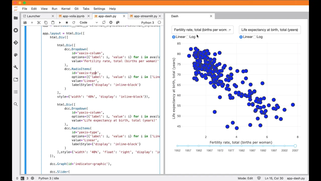
Python dashboard libraries: exploring interaction voila, dash, and streamlit
18.3K
This comprehensive section covers the Python dashboard ecosystem including Voila, Plotly Dash, and Streamlit. Voila converts Jupyter notebooks to standalone web apps using IPython widgets with minimal boilerplate, ideal for incremental enhancement of existing analyses. Plotly Dash uses Flask with explicit front-end/back-end separation, providing maximum customization through HTML-like layouts and declared input-output dependencies. Streamlit offers automatic reactivity and caching for rapid prototyping. The section demonstrates building interactive dashboards from static analysis, adding dropdowns for filtering, and implementing cascading dropdowns where major category selections dynamically update minor category options. Key challenges include converting matplotlib plots to Plotly for interactivity and managing widget callbacks. The progression shows how analysts can enhance their work incrementally, starting from simple filtering to sophisticated multi-widget applications that respond to user input in real-time.
Click to watch →
Deep Dive
Database integration, including querying databases using SQL and loading results directly into Pandas DataFrames.

SQL + Python: Master Data Analysis and Create PDF Reports
61.2K
To load results from an SQL query into a pandas DataFrame, use the pd.read_sql_query() function. Pass the SQL query string and the database connection object as arguments. This method executes the query on the database server and returns the results as a pandas DataFrame, which can then be manipulated using pandas' extensive data handling capabilities. This approach combines the power of SQL for querying with pandas for data transformation.
Click to watch →
SQL Databases with Pandas and Python - A Complete Guide
204.3K
This video demonstrates how to connect Python and Pandas to SQL databases using MySQL as an example, covering three main approaches: (1) Using MySQL Connector to establish a direct connection, create a cursor, execute SQL queries, and retrieve results row-by-row; (2) Using SQLAlchemy's create_engine to create a connection string with username, password, host, and database name; (3) Using Pandas' read_sql method to directly load query results into DataFrames, and writing DataFrames back to SQL tables using to_sql with options like if_exists='replace' or if_exists='append' to handle existing tables.
Click to watch →
![Pandas Dataframes and SQL [How to write dataframes into a sql database/get sql table to dataframe]](https://i.ytimg.com/vi_webp/OjMDXTlVOYU/maxresdefault.webp)
Pandas Dataframes and SQL [How to write dataframes into a sql database/get sql table to dataframe]
57.3K
This video demonstrates how to read SQL database tables into Pandas DataFrames using the read_sql function (which supports both table names and SQL statements with filtering) and write DataFrames back to SQL databases using the to_sql function, with important considerations including specifying index=False to avoid index column conflicts, using if_exists='append' to add data to existing tables (as 'replace' would overwrite the entire table), and the need to install SQLAlchemy for database connectivity.
Click to watch →
Python 201 - Basic Data
13.7K
Pandas can read data from SQL databases using pd.read_sql_query() or pd.read_sql(). For SQLite (file-based database), create a connection with sqlite3.connect(), execute a SQL query, and pass the result to read_sql_query(). For other databases (MySQL, PostgreSQL), install appropriate drivers and manage connections accordingly. The SQL query specifies which data to retrieve, and Pandas converts the result into a DataFrame. This enables reading relational database data into the same analysis framework.
Click to watch →
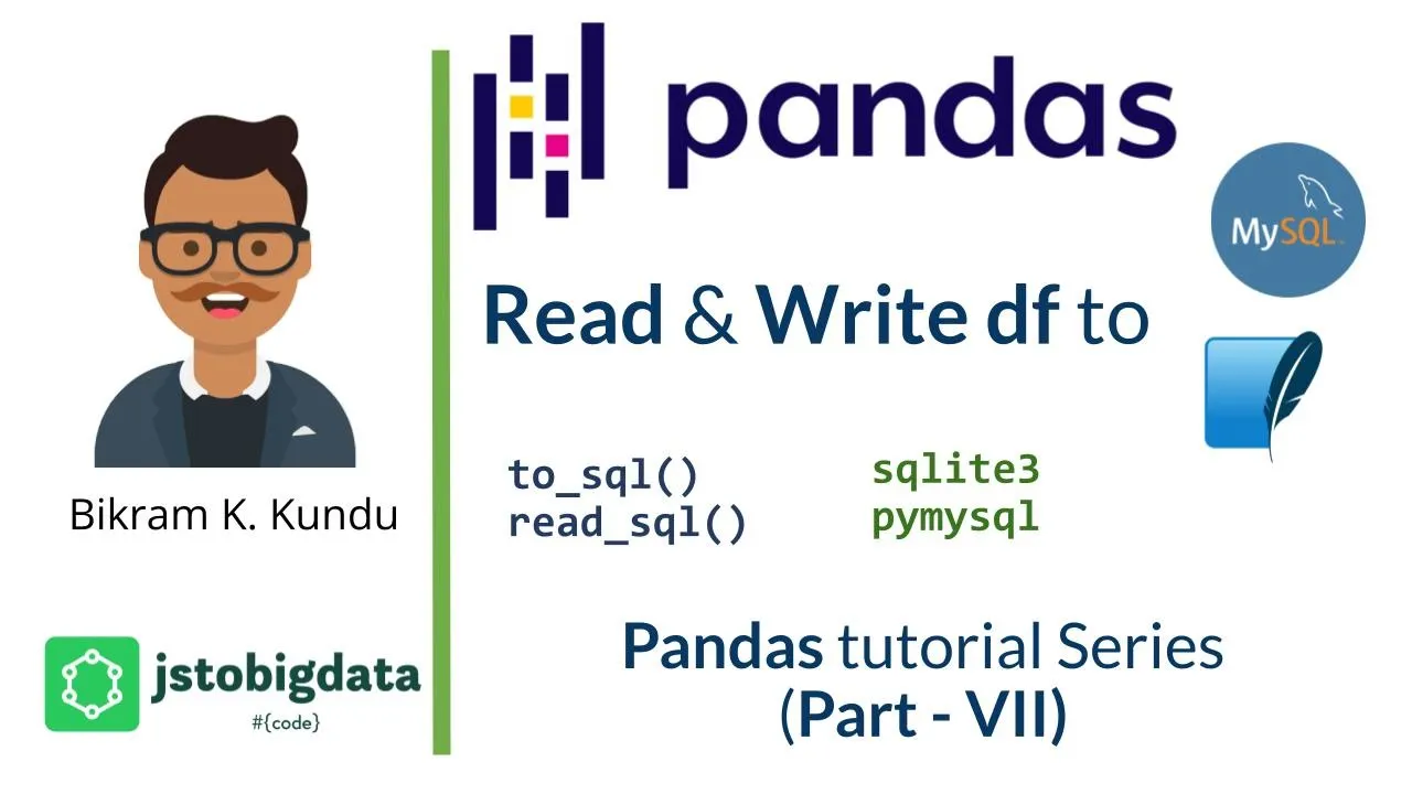
How to handle SQL database in Pandas dataframe - Data Science Tutorial by Bikram Kundu
259
Pandas provides built-in APIs for reading and writing data to SQL databases using sqlite3 for SQLite databases and SQLAlchemy with pymysql for MySQL databases. For SQLite, use sqlite3.connect() to establish a connection and pd.read_sql() to read data into a DataFrame, or df.to_sql() to write data back. For MySQL, create a SQLAlchemy engine using create_engine() with the database URL, then use engine.connect() to establish a connection, followed by read_sql() and to_sql() methods. The read_sql() method accepts SQL queries and connection objects, while to_sql() requires a table name and connection object. DataFrames can have their index set using the index_col parameter during reading or set_index() method after reading.
Click to watch →
Deep Dive
Feature engineering and advanced data preprocessing techniques for handling missing values, outliers, and categorical encoding.

Scikit-Learn Crash Course: Python Machine Learning Library
647.4K
Beyond basic scaling, advanced preprocessing includes polynomial feature generation for capturing nonlinear relationships, and one-hot encoding for categorical variables. Quantile transformer provides robustness against outliers by using percentiles instead of means. These techniques dramatically affect model performance, as demonstrated by comparing transformed versus untransformed data in predictive pipelines. Understanding when and how to apply these transformations is essential for building effective machine learning systems.
Click to watch →
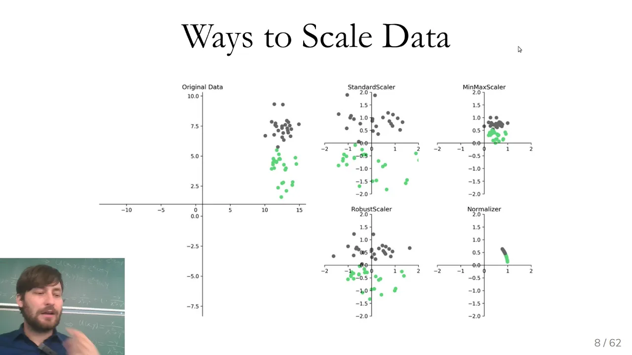
Applied Machine Learning 2019 - Lecture 05 - Preprocessing
9.9K
Categorical variables require encoding since ML models expect numerical inputs. Ordinal encoding assigns numbers to categories but imposes arbitrary ordering that affects model behavior. One-hot encoding creates binary columns for each category, avoiding ordering assumptions but potentially creating wide feature spaces. Pandas' get_dummies() performs one-hot encoding, but requires careful handling of unseen categories in test data. Converting columns to pandas Categorical type before encoding ensures consistent feature alignment. ColumnTransformer applies different transformations to different feature subsets, essential for heterogeneous datasets. For high-cardinality variables, strategies include target encoding/leave-one-out encoding (replacing categories with target summaries), hashing encoding (fixed-size features with potential collisions), and limiting to top N categories. Feature engineering creates new features to improve model performance. Polynomial features create interactions by multiplying combinations of original features, allowing linear models to capture non-linear decision boundaries. Power transformations (Box-Cox and Yeo-Johnson) make skewed data more Gaussian-like, helping linear models and neural networks. Box-Cox applies X^λ/λ (with log for λ=0); Yeo-Johnson extends to negative values. Optimal λ is estimated from data to maximize Gaussian-like distribution.
Click to watch →
DATA SCIENCE ET DÉMARCHE DE TRAVAIL (26/30)
80K
Preprocessing involves: (1) Handling missing values using dropna() or manual removal of mostly-empty columns, or imputation techniques, (2) Encoding categorical variables using OneHotEncoding, OrdinalEncoding, or custom replacement functions with replace() or map(), (3) Removing outliers after initial model creation to avoid premature decisions.
Click to watch →
All-in-one Data Preparation | Missing Values | Outliers | Scaling | Multicollinearity | Encoding
605
Effective feature engineering involves encoding categorical variables while preserving meaningful relationships, detecting and treating outliers using IQR-based methods, and identifying multicollinearity through correlation analysis. Critical decisions include whether to apply preprocessing based on model requirements—statistical models need scaling and multicollinearity handling, while tree-based models tolerate raw data. Making separate data copies for different model types ensures appropriate preprocessing without unnecessary modifications.
Click to watch →

Feature Engineering | Process of Feature Engineering | Great Learning
12.2K
Data preprocessing is essential before feeding data to machine learning algorithms. Data imputation handles missing or incorrect data by replacing it with most common values. Outlier handling uses box plots to identify unusual data points that can degrade model accuracy. One hot encoding converts categorical data (like team names) into numerical data using binary columns. Data grouping makes data more understandable by finding mean, median, or mode. Data scaling brings data to a workable range. A correlation matrix shows relationships between features using color intensity. Diagonal elements are always 1. Underfitting occurs when a model has insufficient data points to train properly, resulting in high bias and low variance. Overfitting occurs when a model learns too much from training data, resulting in high variance and low bias. Both result in poor model performance.
Click to watch →
Deep Dive
Scaling to Big Data using distributed computing frameworks such as PySpark or Dask.
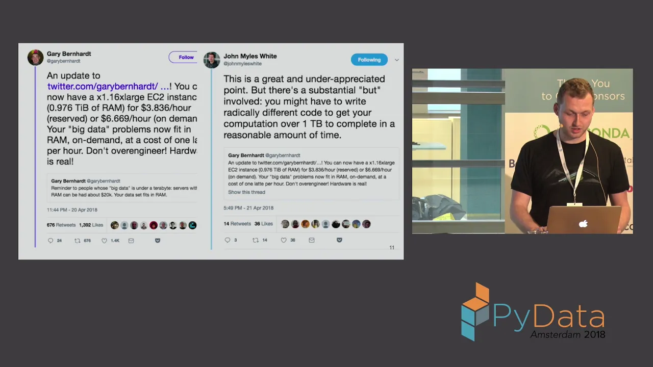
DataFrames: scaling up and out - Ondrej Kokes
566
Distributed frameworks like Dask and Spark enable horizontal scaling while retaining pandas-like APIs. These systems scale by adding nodes, with the ability to scale down to single nodes during off-peak hours. Key benefits include identical APIs for single-node and distributed execution, lazy evaluation that compiles DAGs of operations, and efficient parallel execution. Spark integrates with Python through PySpark, while Dask implements much of the pandas/numpy API. These systems execute actions only when results are needed, optimizing resource utilization across clusters.
Click to watch →
Matthew Rocklin Dask A Pythonic Distributed Data Science Framework PyCon 2017
29.9K
Dask is a Python library that enables parallel and distributed computing by extending familiar Python data science libraries (numpy, pandas, scikit-learn) to handle large-scale data across clusters, using a dynamic task scheduler that automatically manages data locality, resilience, and load balancing through aggressive measurement and dynamic scheduling heuristics.
Click to watch →
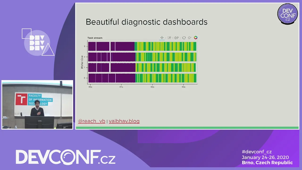
Distributed data workflows: PySpark vs Dask - DevConf.CZ 2020
906
Dask is a pure Python framework for parallel computing that provides familiar pandas-like APIs, enabling Python developers to build scalable data pipelines with cleaner code and better debugging compared to PySpark, which requires transcompiling Python code to Java bytecode and introduces complex error handling; however, Dask performs better than PySpark for single-source operations but lags behind in join-heavy workloads due to its task-based parallelization model.
Click to watch →

Pandas Limitations - Pandas vs Dask vs PySpark - DataMites Courses
37.1K
This video explains how to select appropriate data processing frameworks based on data scale. Pandas handles 1-5 GB safely, up to 30 GB with chunk size, but lacks failover features. Dask extends pandas/numpy/scikit-learn for parallel processing, handling 200+ GB. Apache Spark/PySpark handles petabyte-scale data with distributed processing. Framework selection depends on memory constraints, data volume, and processing requirements.
Click to watch →
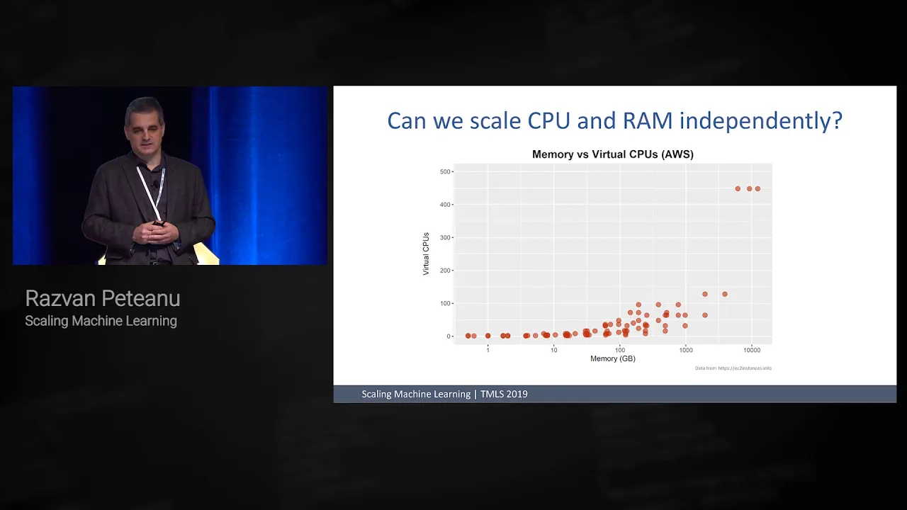
Scaling Machine Learning | Razvan Peteanu
2.8K
Dask is a pure Python framework that scales to hundreds of machines, part of Anaconda with a DataFrame API similar to pandas. It handles data larger than RAM by splitting it transparently across the cluster. Each worker is a separate Python process, eliminating GIL limitations. Dask uses lazy evaluation where transformations execute only at the final step, with a task scheduler tracking dependencies and data movement. It can register as a Joblib backend, allowing scikit-learn to delegate parallelization without knowing work is distributed. Dask provides excellent visualization including a task stream showing real-time parallelization effectiveness, where white indicates idle cores (bottlenecks) and red indicates network data shuffling.
Click to watch →
Course Overview
Target Audience
Learning Outcomes
Practice & Project
Prerequisites
Course Overview
0:00- 1
Practical, beginner-friendly data analysis course.
- 2
Live online with verified certificate option.
The R Ecosystem and Tidyverse for Data Science
While Python is a general-purpose language adapted for data science, R was built from the ground up specifically for statistical computing and visualization. For students learning data analysis, the R ecosystem—particularly the "Tidyverse" (which includes dplyr and ggplot2)—offers a highly cohesive, intuitive, and mathematically rigorous alternative to the NumPy/Pandas/Matplotlib stack. Unlike Pandas, which is often criticized for its inconsistent syntax and heavy memory overhead, the Tidyverse is designed with a unified philosophy that makes data manipulation and exploratory data analysis (EDA) highly readable and expressive. Furthermore, R remains the gold standard in academic research, bioinformatics, and advanced statistics due to its superior out-of-the-box statistical modeling capabilities. Learning R provides a distinct, data-first paradigm that contrasts with Python's software-engineering-first approach, broadening a student's perspective on how to interact with data.
Basic Python programming syntax, including variables, data types, loops, conditional statements, and custom functions.
Fundamental mathematical and statistical concepts, such as mean, median, standard deviation, and basic probability.
Familiarity with tabular data structures, such as spreadsheets, and common file formats like CSV and Excel.
Basic usage of a Python execution environment, preferably Jupyter Notebooks, Google Colab, or VS Code.
Introduction to Machine Learning concepts and predictive modeling using the Scikit-Learn library.
Advanced data visualization and interactive dashboard creation using libraries like Plotly, Seaborn, and Streamlit.
Database integration, including querying databases using SQL and loading results directly into Pandas DataFrames.
Feature engineering and advanced data preprocessing techniques for handling missing values, outliers, and categorical encoding.
Scaling to Big Data using distributed computing frameworks such as PySpark or Dask.
3.2M views73.6Klikes9:56:22@freecodecampOriginal Release: 2021-02-18
Data analysis with Python Zero to Pandas is a practical beginner friendly and coding focused introduction to data analysis.
This is a live online course and you can earn a verified certificate of accomplishment by completing this course if you are interested in learning data science with python but don't know where to start then this course is designed just for you you can learn more and register at xero2pandas.com.
By the end of this course you will be able to confidently use the python programming language and its amazing ecosystem of data science libraries like numpy for mathematical and statistical computing pandas for data processing and analysis matplotlib for creating beautiful visualizations and much more you will get a chance to practice and improve your skills with weekly assignments and you will also work on an end-to-end course project where you will perform data analysis on a large real-world dataset this is a beginner-friendly course so you don't need to have any prior knowledge of python or data science some basic programming knowledge will be helpful. But don't worry if you don't know programming you can learn these concepts with a little extra effort.
Up Next
20:00
Python Pandas Time Series: DateTime & Timestamp Data Tutorial
@joejamesusa
14.6K views•2020-06-17
87:26
Introduction to Secure Multiparty Computation with Yehuda Lindell
@fhe_org
7.7K views•2021-02-04
85:36
Rust Programming Tutorial for Beginners: A Comprehensive Guide
@freecodecamp
354.1K views•2021-11-30

19:25
Enigma Machine Mechanics: WWII Encryption Explained
@JaredOwen
13.2M views•2021-12-11
Related Study Plans & Knowledge Roadmaps
Structured learning paths in Computer Science
computer-science
Container Runtimes: Namespaces, Cgroups & Go
01Linux Systems & Go Programming Foundations
02The Core of Isolation: Chroot and Filesystems
03Linux Namespaces: Process Isolation
+ 3 more learning modules
32h6 modules
Explore Roadmap
computer-science
Building a CHIP-8 Emulator: Rust & CPU Basics
01Computer Architecture Foundations (Bits & Bytes)
02Rust Programming for Systems Development
03CHIP-8 Virtual Hardware Specifications
+ 2 more learning modules
32h5 modules
Explore Roadmap
computer-science
Building BitTorrent: Go, P2P & Concurrency
01Go Fundamentals & Concurrency
02Networking Foundations & P2P Architecture
03Bencode Parsing & Torrent Metadata
+ 3 more learning modules
26h6 modules
Explore Roadmap
computer-science
Actor Models (C++ Concurrency & Lock-Free)
01C++ Multi-Threading Foundations
02Thread Pools and Task Scheduling
03Atomics and Lock-Free Queue Design
+ 3 more learning modules
45h6 modules
Explore Roadmap