











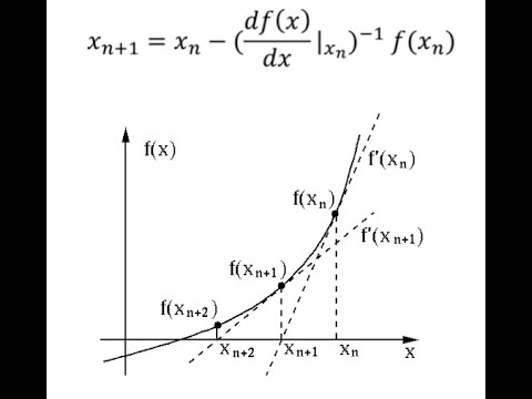








The Newton method is an iterative root-finding algorithm that uses tangent lines to approximate roots of a function; it has quadratic convergence (error reduces by the square of the previous error), making it significantly faster than linear methods like bisection, but requires the function to be differentiable and faces reliability issues such as potential divergence or oscillation if the derivative is zero or the initial guess is poor.
Newton-Raphson Method: Root Finding & Convergence Order
Added:Differential calculus, specifically the concept of derivatives and the geometric interpretation of tangent lines.
The fundamental concept of root-finding for non-linear equations, including basic interval-halving methods like the Bisection Method.
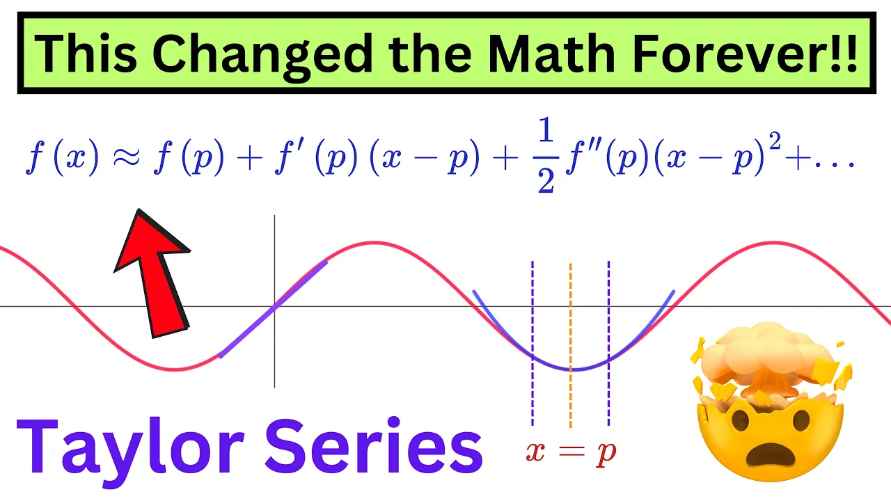
Taylor Series expansions (specifically first-order Taylor approximations) used to derive numerical formulas.
Basic arithmetic operations with complex numbers and representation of roots in the complex plane.
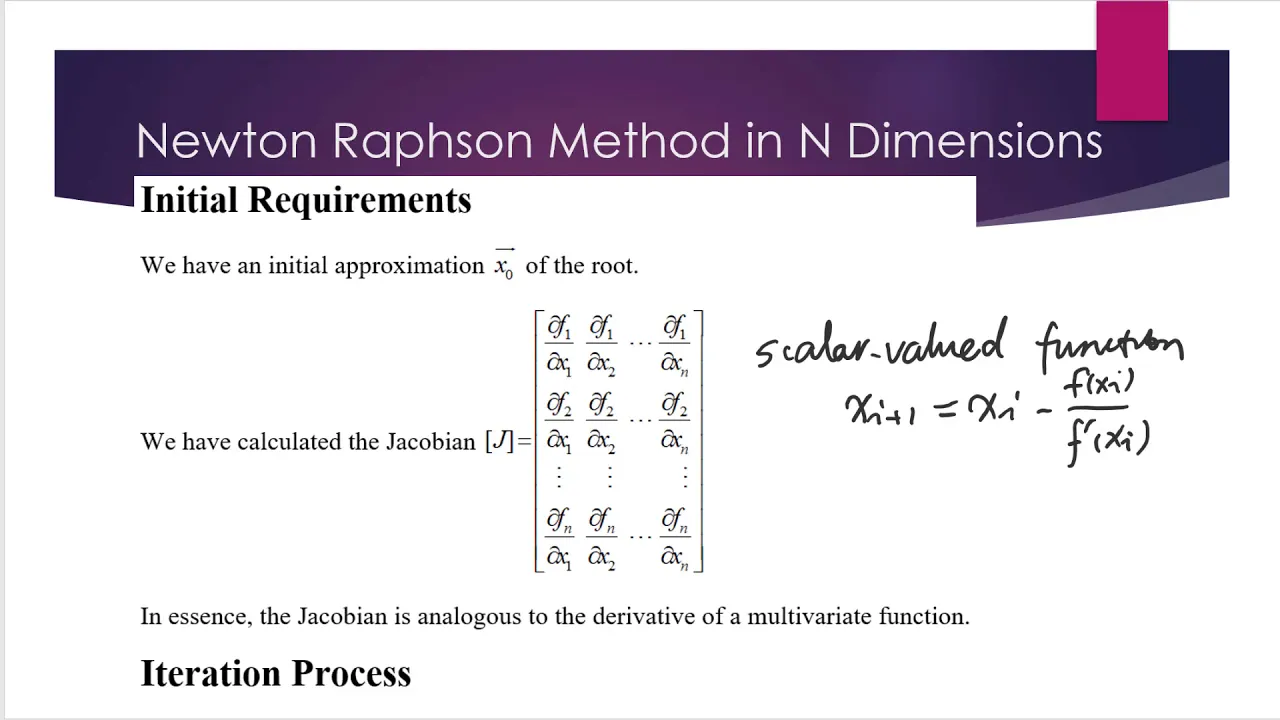
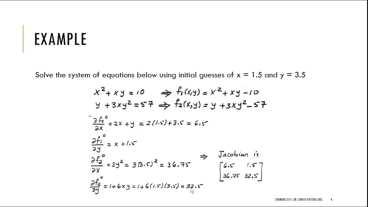
The Multidimensional Newton-Raphson method for solving systems of non-linear equations using the Jacobian matrix.
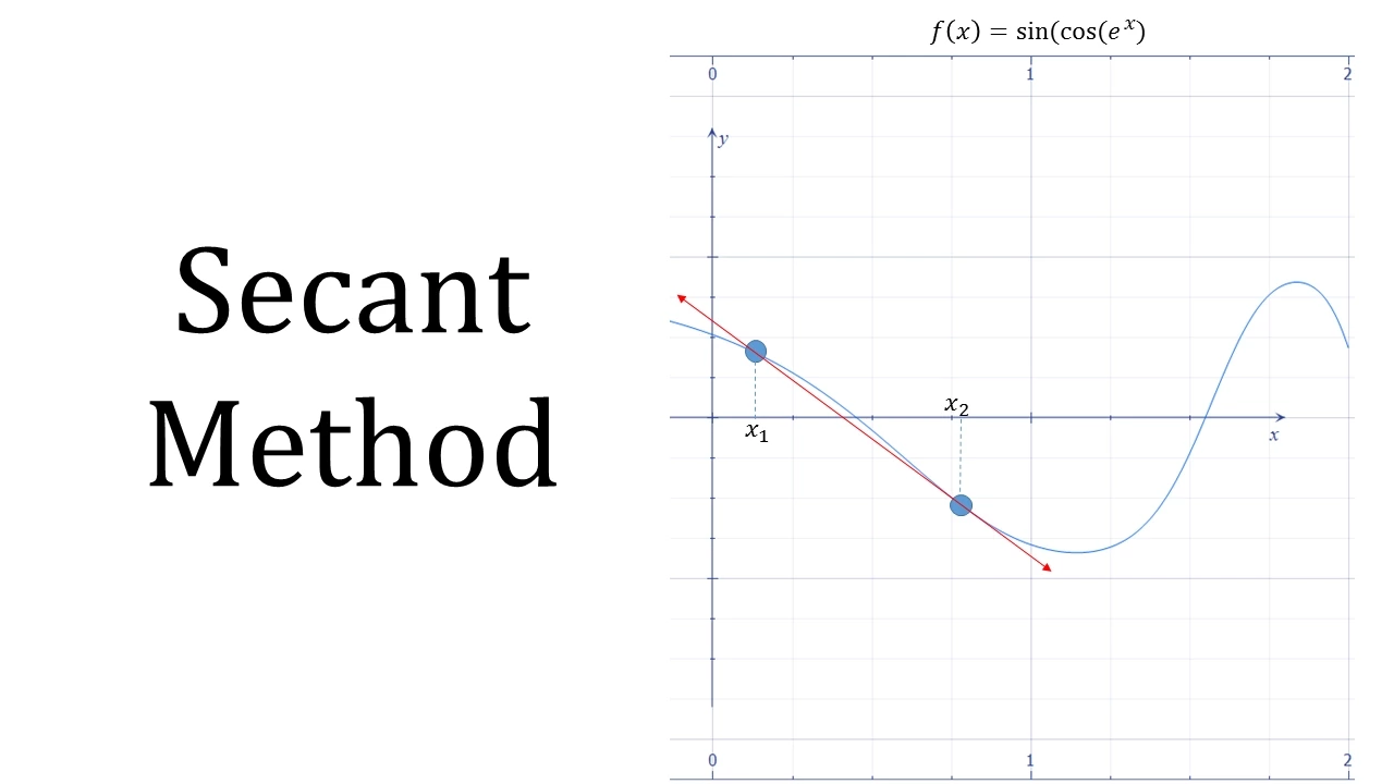
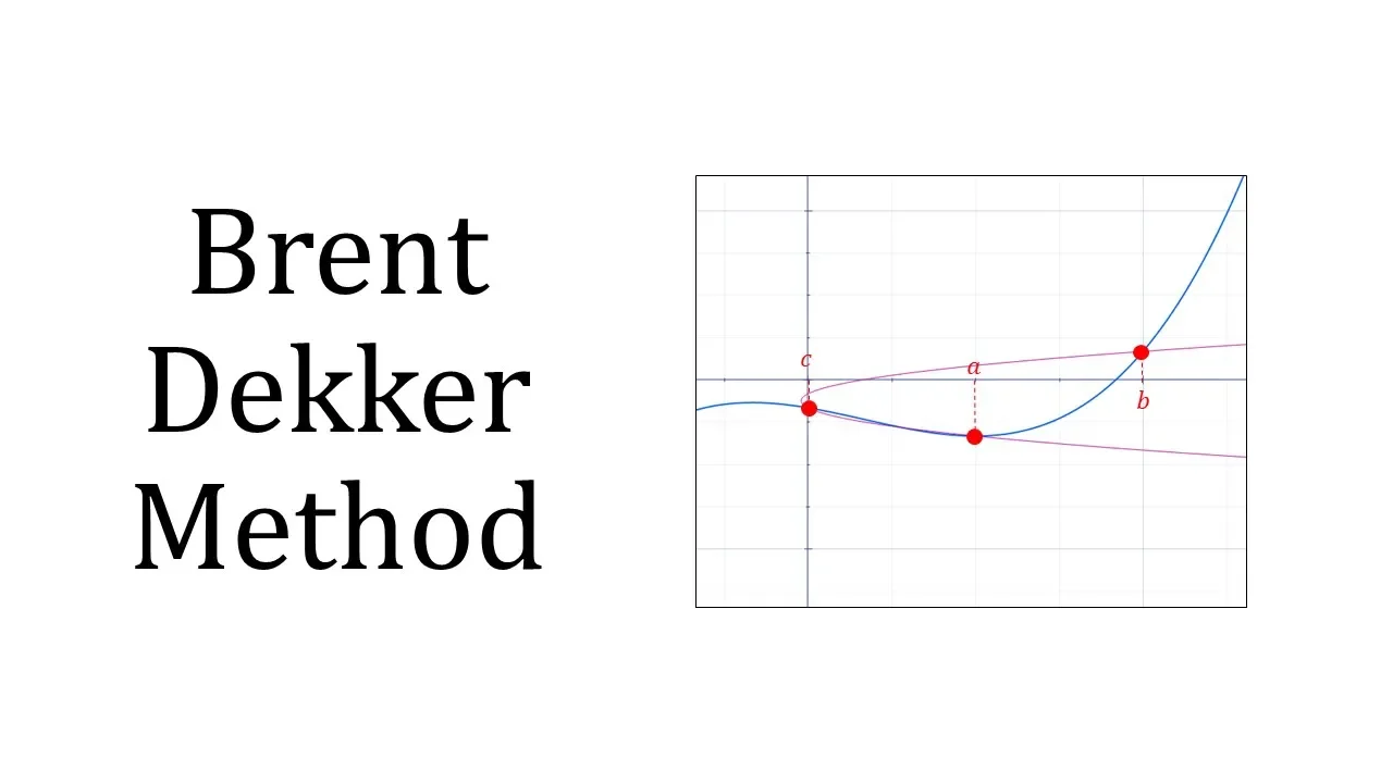
Alternative root-finding techniques that do not require analytical derivatives, such as the Secant Method and Brent's Method.
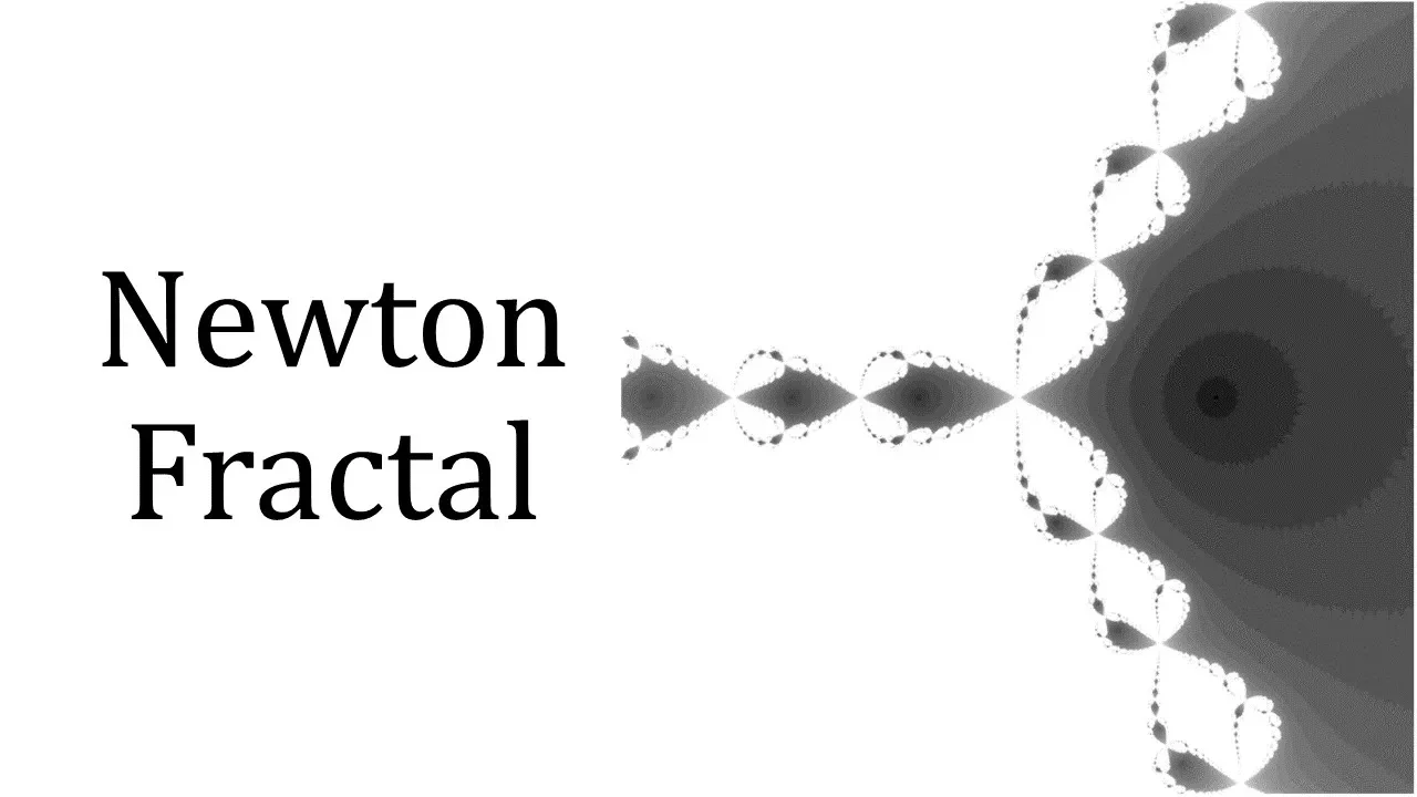
Newton's Fractal and the chaotic behavior of the method when analyzing convergence basins of complex polynomials.
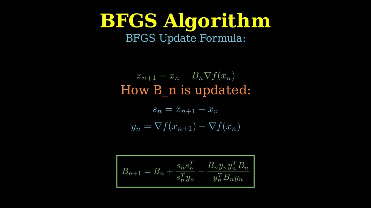
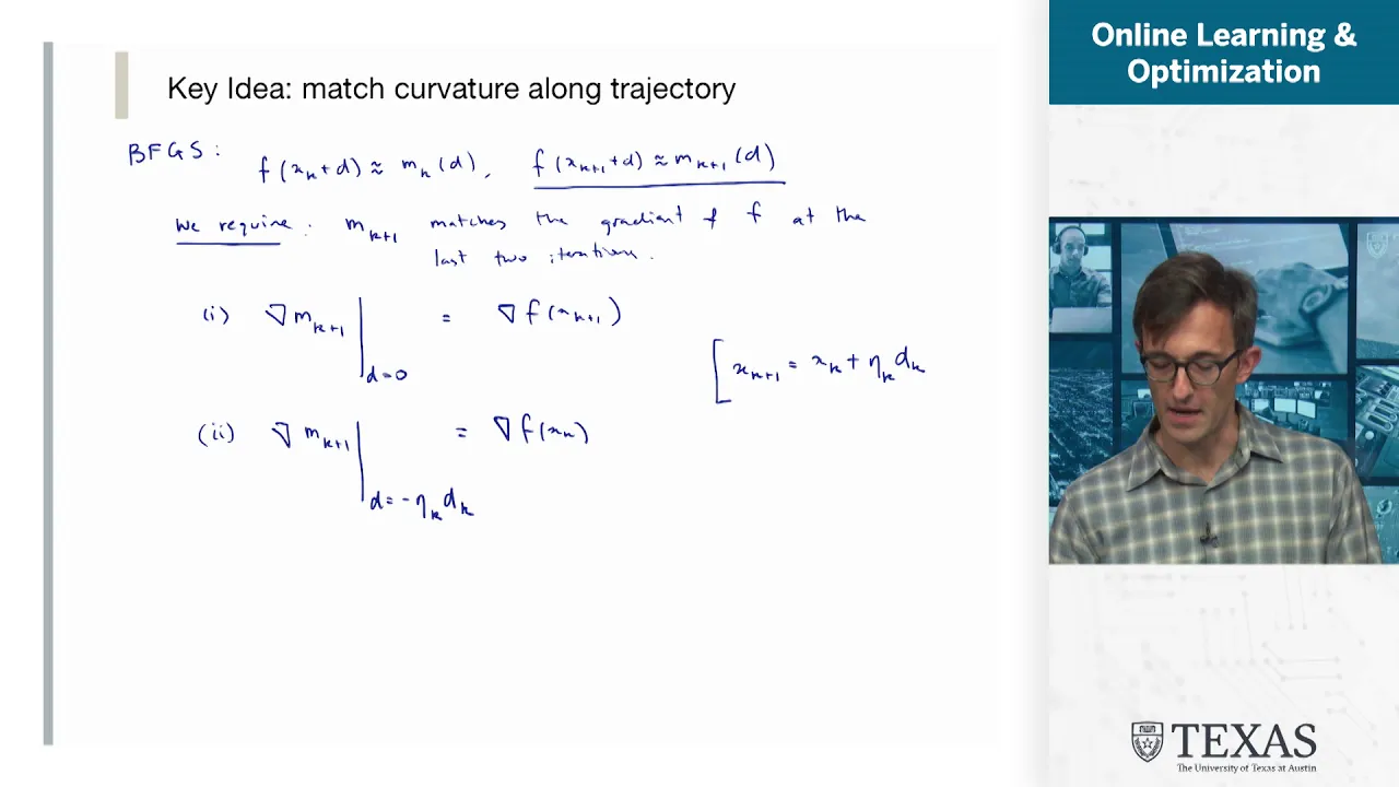
Quasi-Newton optimization algorithms (such as the BFGS method) used to find local minima and maxima in machine learning.
198 views2likes1:04:50Original Release: 2024-04-28
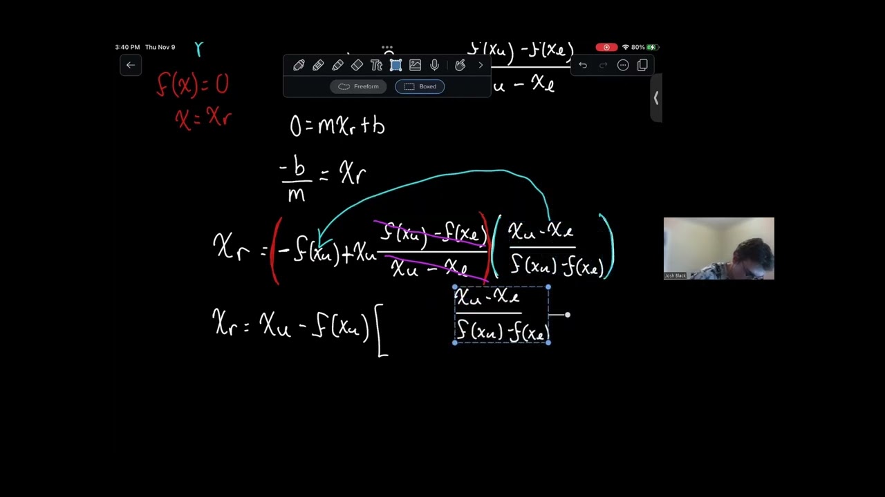
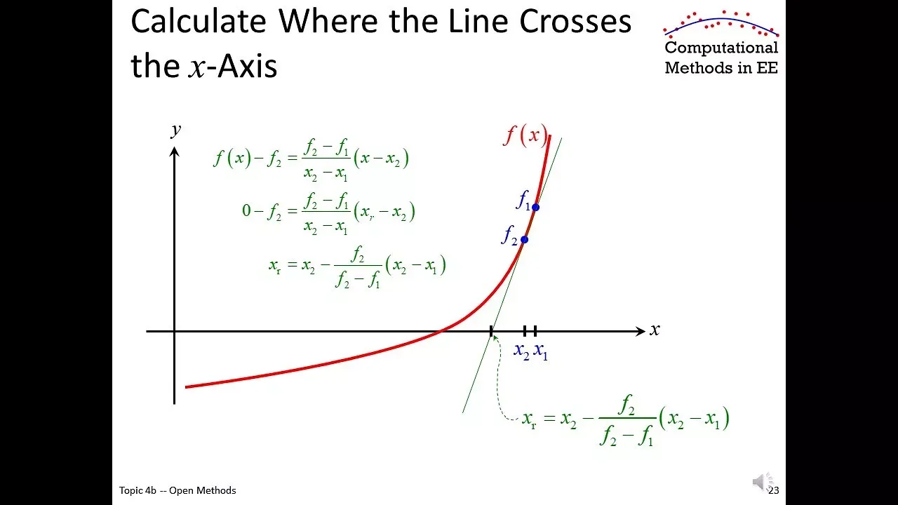
okay so a new beginning I have a function I'm trying to find a root so I just shoot some number and now we want to take into account the shape of the function so let's say that the value is somewhere here and let's say that the function goes like that now I'm trying to get to the root which I can see over here and when you look at this picture you might say okay uh I'm sitting here so presumably I have a lot of information about a function at that particular point and perhaps I could take the tangent line and if I take the tangent line it must intersect with a little bit of luck the xax and I think navely that it's a better estimate and I'm sitting here now did I get closer to the root yes does it look like a good idea I think so let's try it again I take the tangent line and I got so close to the root that I cannot even write the name of the new number properly so this looks like a killer method this looks good and the next tangent line I cannot even draw the picture properly that's how close to the root I get so this looks like a very nice method let's try it our test function is X Cub - x - 3 and let's say that my initial guess is 5 so we already calculated how much is a five do I remember it I think it was 110 125 12 oops there was 10 here got carried away sorry there was 10 here 25 20 110 yeah where do I get the tangent line I don't feel like doing it each time again and again so let's do it in general I have some point here which I'm going to call XK and I'm sitting here and then the value the elevation is fxk and of course we know the slope the slope is the derivative of F at XK that's the data that I need I have a point through which the line goes which is here and I have the slope I can write down the equation the tangent line well there are several ways how to write equation of a line probably each of each has his own or her own preference my preference goes like that at a certain X the elevation on the line is given by the original elevation and now there is the slope and there's the movement along the x-axis that's how I prefer to see a line okay uh let's see that's a tangent line and I'm looking for the intersection with the x-axis which means I am putting y equal to zero so I'm going to rearrange it somehow and solve it for X so I will move FK to the left hand side and then I divide by the derivative so minus fxk over frime XK is equal to x - XK and then I move XK to the left and I get a nice formula so that's my new XK in this case it's XK + 1 that was nice and easy okay let's use it so I need a derivative at XK what's the derivative it's 3x2 - 1 so when I'm sitting at the point 5 the derivative at 5 is 25 * 3 is 75 74 I was hoping for something better because now I have to divide ah it's going to be ugly okay that's life what's X1 X1 is 5 minus 110 over 74 which is 5 minus I don't like it 37 by on the top 55 this is divisible by five and this one not this is divisible by 11 and this why isn't um that's it well I guess I could use a common denominator but I don't feel like it 5 * 37 okay that's okay good enough for me so that's X1 and now we should calculate x2 in the same way and so on you can easily imagine how the calculations would go uh again why am I doing it by hand first of all we get to appreciate the works workings of this algorithm second of all we are preparing for the exam because on the exam it may happen that you are given a function you are given a starting point and you will be asked to show how the Newton method goes by the way the same can happen with the bisection method I can give you a function a starting interval and ask you to show me several iterations by hand to show me that you actually know the workings of the algorithm or perhaps I could ask for the explanation of the algorithm with a picture I can ask for this procedure I can ask for explanation of the bisection algorithm these are two basic algorithm for this course and I want you to know them quite well back to the question by the way there is a third reason why I'm doing it by hand it's a tribute it's a tribute to people who let's say even in 1950s were sitting somewhere with huge sheets of paper and pencils and doing calculations like that for life because at the time the computers were not widespread they were just starting and until all the way up to let's say 1950s people were doing calculations like that by hand and now we can appreciate that it was a really hard job by the way these people were called computers so uh yeah we are lucky but anyway we can appreciate that they wanted an algorithm which runs fast you don't want to spend half a month doing calculations like that definitely not so is this algorithm fast that's a good question uh first we are going to give it a name this is commonly called Newton algorithm but there are also some other names for it and I'm not going to take sides on any names if I had my way I would call it a tangent method because we are using tangents yeah tangent method everybody would know what it means but it's called Newton method or Newton raone method yeah I don't want to go into it anyway here we go we have a function which is continuous and it must be also differentiable otherwise we are in big trouble with the formula so it must be also differentiable and we have a tolerance we just choose some X note just shoot from the hip some number but if we for instance can plot the function we can make an educated guess which would be better but it's another story okay we choose some X not it becomes XK for k equal to Z and then there is a Formula which tells us how to calculate the next approximation and by a remarkable coincidence it's exactly the same that I have here so I was good okay uh uh let's skip the next part yet so we have the procedure it's called the Newton method now what can we expect from the Newton method let's make a little comparison and let's make a little experiment as well so I have a little code here let's make it larger again so here is a code I'm asking for the root of our function f I'm starting at zero for some reason uh I started here at five let's start at five and I'm using the Newton method and the tolerance is 0 point well that's 10 to4 just like I did before with the bisection method let's fire it up wow just six iterations that was nice that was very nice let's try 10 to -7 wow just six iterations is that weird is there some error probably no actually the quality improves so far that if we ask for three digits correct essentially we also get seven right away there is no reason for newon method to stop earlier because the Improvement is so vast in just one iteration if it stopped in iteration five then the error will be larger than 10 to4 and the next iteration already has a very nice small error so that's a wickedly fast algorithm let's put it here fast reliable reliability well unreliable unfortunately what can go wrong well first of all technical problems if you don't have the derivative you are out of luck it may also happen that you are happily running using your tangent lines and then suddenly you find derivative equal to zero which means means horizontal tangent line of course horizontal tangent line will never intersect the x-axis you're out of luck these are not fatal problem I mean this is not a fatal problem you can just start at a different place with your X note and you hope that you will not reach this place so in practice this is not such a big problem but there is something else uh first of all the Newton method as it goes by the tangent lines jumping around the graph it likes to one let's start at zero now perhaps first let's have a look at this column with XIs we started at five and we very steadily went all the way to 2.3 and so on if I started zero that was unexpected probably let's have a look at it from zero we go to -10 why I have no idea the root is not there anyway then it it goes back to zero and then it jumps all the way to 65 and then it goes to zero again then it goes to four so it overshoots and then it settles down to 3 2.3 and so on so it was going left right and so on yeah it likes to walk around you know take a look at the countryside and so on that's typical of Newton unfortunately uh it can get even worse imagine this uh imagine that there's an SYM toote but the function never actually touches the x-axis here now if you're unlucky your initial guess will be here and the Newton method will go here and here and here and so on it keeps taking tangent lines and goes all the way to Infinity it never goes to the root R another bad shape is C if you are really really unlucky with your initial guess your tangent lines start jumping right here moving left and right in the saddle you will never get out to reach these roots so essentially when you are using the Newton method you should be careful and you should watch what it's doing so we definitely want to have some bound on the numbers in the calculations so there is one of the things which is Incorporated in the procedure that I'm using if the the numbers get too large the procedure stops and tells me about it and then it's up to me whether I want to continue or not I have to make the decision I as a human being the same thing is here there is a restriction on number of iterations and if by a certain stage we don't get a rout uh the procedure stops automatically and of course I can change this bound so if I feel that I'm on the right track I can say okay go longer but I have to control the Newton method here is another nice example square root of x we all know square root of x now let's imagine that I create a function by flipping it around twice so this is an odd function now what's so special about it if I start here and I make a tangent line then my picture is not okay it's too flat I ran out of room okay but in the actual picture which would would be correct the tangent line intersects at exactly Nega XK and by the Symmetry when you make the next step you go back here so when you start the Newton method on this function it will just go left right left right left right never stopping so you can easily throw off the Newton method it's unreliable on the other hand this picture looks really nice we started and yeah looks very nice so there are some circumstances and of course mathematicians are curious people and they like to have certainty in situations so they were able to identify situations when the uh Newton method actually converges uh just to give you some example here we go to the slides so I'm not really going to work with this theorem so it's up to you just to read it and see what are the uh inputs it so we have a functional interval where it changes sign which is actually here that's a good news and now on this interval there are some assumptions and if you translate these assumptions into ideas what you learn is that on this interval the function must have a good enough monotonicity and a certain concavity it has to be concave up or concave down doesn't matter which one but it has to choose one and stick with it we don't want see the function to wave and then if you get lucky with your initial guess you are guaranteed to get the answer which is the last line it says the sequence generated by the new method converges to a root so in some situations we are guaranteed to get the root but it's not easy to get to them as you can see in the picture uh What people actually often do is to combine these two approaches we have a method which is slow but it's reliable and another which is unreliable but hopefully fast we will talk about it later so what people do they start with a bracketing they narrow down the route but they they are not going to go to extremes they just narrow it down reasonably to get a nice situation and in the nice situation you apply the newon method and you get very fast a very good approximation so there are different strategies that people use anyway let's go back uh unreliable in some situations there is a theorem error control no error control and that's pretty serious but again that's typical of numerical analysis we don't know the right solution so if we don't know it how can we specify or calculate the error uh that's a problem what's the data here we have some function and we have some points on it how do we find the distance to the actual root well essentially we cannot so that's a big problem uh there are some uh tricks that can help sometimes or some situation that can help uh let me show you one it's called fact because it's actually fairly simple and let's translate it into ideas we have a function we have a root and there is a neighborhood of a root where something happens now what is happening on the neighborhood the function is differentiable there so it's nice it's smooth it doesn't break sharply and the derivative is bounded away from zero we are pushing it up using some constant m one and this constant M1 should be positive you'll see why so here's the picture there is a root and something pushes the derivative away from zero what does it mean well practically speaking it means that the function has to be rather steep it shouldn't be flat because flat functions have very small derivatives now what does it say uh we take take some approximation of the root which is over here and we get some value now remember the technical assumptions this inequality M1 is less than or equal to derivative they tell me that the function is going rather steeply down or up we don't know in this picture I want to see an increasing function this picture because it's supposed to have a root here remember so it's increasing so it's very sharply increasing if it's sharply increasing it cannot go like that it's forced to go at some angle which can get also larger we don't know there is no bound from the top but the important thing is there is bound from below so the flat Nest is forbidden this functions to grow at a certain rate at least even faster now if I know this distance and if I know this extreme Bound for the flatness I can calculate from here the maximum possible error the maximum possible distance between the approximation and the actual root that's the geometric idea now how do you prove it the answer is very simple you just apply the mean value theorem to this interval r r head let's try mean value theorem How does it go like that f r minus f r head divided by R minus r head is derivative at some mysterious Point s now we are going to apply absolute value so I'm applying absolute value here I'm applying absolute value here and also here now the mysterious Point Cai happens to be between R and R head so they all live in this neighborhood U so definitely the derivative is bounded From Below by M1 now you can see but it's useful to have bound From Below we are pushing this whole thing up now I can move R minus r head to the right I can move M1 to the left and I get the following I get that R minus r head is bounded from above which is the useful bound and that's actually the error of approximation by 1 / M1 and this difference but actually R is a root so this number is zero so there is the value so if we get lucky and we get information about the derivative then we actually can compare the actual error and the value of the function so how do we know when to stop well we simply wait for this number to be less than Epsilon and we are done so that's nice and it's actually also a nice reminder of the mean value theorem which is also nice uh but in applications you very often don't have this information so it's not that nice so what do we have in general and the answer is uh nothing really so how do we know when to stop well we guess so what people do there are three traditional stopping Condition it's called stopping condition let me put them here the first stopping condition is the absolute difference when you calculate the next approximation XK you ask how much it differs from the previous one and if they differ just by a little bit you can get optimistic and you can say okay so I'm probably close to the root but of course that need not be true unfortunately but it's probably the most popular stopping condition uh sometimes people work with relative difference this makes sense if the approximations are really really really huge it does not really work well if those approximations are are close to zero but sometimes people use relative Difference by the way in books people call it absolute error and relative error but I don't think that's a good name because it suggests that it somehow that it has some connection with the actual error of our solution it does not have any connection with the error of our solution uh the last stopping condition that people ose is the value that's also fairly popular and you can see the reason why because if you get lucky there is a relationship between the value and the error of your approximation but unfortunately since we don't know M1 in applications we don't really know what's the actual relationship so also the third condition although it looks like a good idea actually does not work reliably uh what we don't really like in all these pictures is flat functions first of all if the function is flat then we cannot make a good bound on the derivative from below and the relation relationship between the value and the error gets really mky there there could be a big difference between them so the last condition doesn't really work well in particular imagine that the root R is a root of higher multiplicity roots of higher multiplicity have this unfortunate property that the derivative there is also zero so in fact we cannot make a reasonable lower estimate the only estimate that works is zero and if we put zero here we get infinity and nothing useful comes out of it so again the second time we see it roots of higher multiplicity cause troubles they are really bad uh and also you can think of this picture that's a function which is very flat it has a root R over here now I started here and I'm doing let's say the tangent line method the Newton method but this actually applies to any iterative method there are many methods that are looking for the root and most of them has the form that we are producing successive iterations successive approximations and they all share the same problems how do we stop how do we control the error so some method I don't care which one it's approaching the function approaching the function and we are waiting for the value to be small which happens let's say here but we are still very far from the actual root so the third condition is also not very good so none of the three conditions Works reliably which uh people sometimes solve by let's say using the first and the third they want both of them to be true and they are hoping that things get good but they won't that's a problem so I'm looking at a function which is actually e toga X and I shift it down by a little bit so it does have a root I asked for stopping condition or stopping Criterion to be the value so this run stop after two iterations and suggests that perhaps 2.99 which is like three so perhaps three is the root is that true how do we find out we don't have any control over the error there is actually a fairly simple test and it's a common sense test let's say that you are trying to find an approximation and you come up with some number but now you are supposed to somehow guarantee that the error of this approximation is less than Epsilon can you somehow guarantee it well you can try this thing you move to the right and you move to the left by Epsilon and you substitute into a function now if you get lucky you will see different signs and if you can see different signs then you are guaranteed to have the actual root here and the error is definitely less than Epsilon so that's a very nice simple test and I'm actually quite fond of this test test because you don't need any special theory for it you don't need any special tools you can use it with any method each time you come up with approximation of a root you can simply test and if you get lucky you get confirmation that your guess is good now if you have unfortunately the same signs this can happen then this doesn't mean anything because the root can be here if the function goes like that so again it's a test which is not perfect it's not an equivalent test it just gives you good information if you're luy otherwise it doesn't give you any information and as usual case of Parabola this test doesn't work well for roots of higher multiplicity but anyway let's try to apply it here so I'm going to store this answer this 2.99 something and I'm going to evaluate at the root and also I shift up and down by 0.1 because that's the tolerance that I'm using here I'm not I'm very tolerant here 0.1 not a good Precision anyway uh I got three positive numbers which is not very good news it could be that the root is there but I know that it's not there because e tox we know how it looks like it's a function that looks like this and I shifted it down so there is a root so let's try another what if I put the relative error this time the algorithm run a little bit longer now is it a good news or bad news that's a good question now by changing the stopping condition I am not changing the numbers which are produced by the algorithm so when I was running the value stopping condition we got the same three numbers these three numbers now if the algorithm is doing its job well the successive numbers are actually better approximations of the root so if the algorithm runs longer with more steps it's actually giving me a better answer so in this particular setting short run means lower quality of the approximation so I don't want shorter runs here I got a longer run so I think that this approximation is better now I used relative error what does it mean I'm essentially asking for the absolute error to be less than Epsilon but not by itself I'm dividing it by the approximation which is about eight so I'm taking the absolute error dividing it by eight asking it this well actually this is the thing this is not the error this is the difference let's call it D this is the difference between the last two approximations the difference between last two approximations divided by approximately 8 is less than Epsilon that's the condition which got triggered in the last line and I have approximation 8.5 now is it a good approximation let's run my test again I got three positive numbers so I'm still still here I'm still here on the curve I didn't get far enough now what happens if I change this condition to Absolute difference let's think about it the relative difference is dividing uh this Distance by eight so I'm helping it to get small I'm helping it to stop earlier if I remove the eight I am forcing the algorithm to work harder so generally I expect a longer run in this case when I'm dividing by a number larger than one that's important so I expect a slightly longer run let's see yeah 11 iterations before it was eight I think so I got a new estimate let's have a look at it is it good enough yeah I got a change of sign as you can see so now I know for sure that there is a root within 0.1 of this approximation so you can see that in this particular example the absolute difference worked best but there are examples when it doesn't work best so you never know okay by the way let's say that for some reason we decided to stick with the relative error and we found that the Run wasn't long enough can we help it the answer is yes we can change the tolerance but only in the procedure so we force it to run longer so I improved the tolerance by one zero I lowered the tolerance 10 times I'm forcing the program to run longer and the new result but checked with the original Epsilon because that's what the customer wants so now yeah now I got confirmation there is a change of sign the last two values so now I know for sure that I reached the right approximation it's good enough okay so this is a very important question of stopping conditions three of them none of them reliable so we are just playing it by the here and there is this little test which I really like uh surprisingly enough I don't find it in books typically uh okay so that's the error control fast let's talk about the speed of the algorithm uh we need room let's talk about the speed of convergence uh that's actually a fairly general question imagine that we have a sequence and the sequence converges to some number and we can ask that's a natural question how fast does this convergence happen and when we think about it we can just look at the difference and ask how fast does it go to zero so we can focus on sequences that tend to zero and introduce some notion that would measure the speed of convergence now in the context of numerical analysis we would call this EK that's the error but we can simply see it as a the difference how do we measure speed of convergence and it turns out that a good idea is to compare Improvement of one iteration or or one step in the sequence we look at the error at a certain stage we look at the next one we compare them we did exactly the same in that experiment in the chart that we can see over there there we actually asked for increased precision and we asked how many iterations it took but the same experiment can be interpreted the other way around we can look at one iteration and see the Improvement and uh it's natural to somehow compare the errors and we saw something like that before when we were exploring the bisection method we saw that the error k + one was bounded by 1/2 of the previous error actually there we talked about the estimates for error but let's keep it simple let's imagine that these are the errors now that's the kind of relationship that looks hopeful let's see in general we would like to explore comparisons like that now let's make a little experiment about the impact of such a relationship on the error so we start with error AK or EK which is 10 to -4 which is 0.1 2 three zeros and one what happens after we pass to the next stage to k + 1 well e k + 1 which is divide by two and we get 0. and divide by two so it's 05 let's make the next step uh okay how much room do I need about this much so let's have a look at the error EK + 2 it's 0 point 1 2 3 4 zeros and then 25 we talked about correct digits so just out of curiosity we have three correct digits here four here and four here now we know that with bisection we can expect three correct digits for every 10 iterations so that gives us sort of like a an intuitive understanding of the speed of convergence and we commented that this is really slow so let's say that we want a faster convergence how can we force it and the natural idea is that we make C smaller so let's say that we can somehow arrange for this inequality to become uh let's say 1 over five that's a nice number to work with for instance we can take bsection we can take the basic interval but instead of dividing it into halves we can divide it into five five sub intervals and pick to one where the sign changes uh Quin section whatever okay so we just imagine a method like that now how would the error react to such a relationship again we start with 10 to4 so we have three correct digits then we divide by 5 we get o0 Point O O2 four correct digits and then for the next stage we still have to divide by five so it's 0.1 2 3 4 and now we divide by five here and we get 04 so it's five digits well it seems that we are getting one new digit with every iteration uh actually it breaks down after a while we can make an analysis similar to the one that we made for bsection and it turns out that for every 10 iteration ation to get seven new digits correct so this is a definite Improvement here it was three per 10 here it is seven per 10 so it's better but it's still not a speed demon because you are still adding new digits as a as a steady rate essentially and it turns out that this is not enough we can do better so the constant C is not the place where we we should focus we should focus on the exponent now we can say okay there is no exponent well there is there's exponent one in general I can try to raise it by some means and we will talk about it soon so just out of curiosity let's imagine that we can somehow improve power 1 to power 1.5 and I'm going to ignore this constant to make my life easier and in fact it's not really crucial we will see it soon so let's imagine that there is power 1.5 here which is 3 over2 so we should take square root and then Cube the starting error is 0 point one 2 three zeros and one just like before okay the next error we take square root which is 10 to -2 and we raise it to^ three which is 10 to -6 uh perhaps I will make a little note here this is 10 to -6 which means five zeros 1 2 3 4 5 and one the next stage we take square root which is 10 to -3 and we Cube which is 10 to 9 so it's eight zeros 1 2 3 4 5 6 7 8 and one so when you look at the number of zeros now it goes 3 5 8 and if you try the next step it will be even more the difference between the two successive number of zeros so here the zeros or the correct digits are not increasing in a linear fashion but much faster this is a much better convergence of course the question is whether we can find a method that works like that very good question let's be super optimistic let's imagine that we can find a method which actually has uh exponent equal to two what happens well the start of error is 0.01 just like before three correct digits we Square it and it becomes 10 to8 so it's 0.1 2 3 4 5 6 7 zeros and one and then we Square it again this becomes 10 to -6 0 point 1 2 3 4 5 6 7 8 9 10 11 12 13 14 15 1 okay 15 correct digits and you can see that the number of correct digits actually doubles or better than doubles with every iteration now if of course it may happen that there will be some constant C which may slow it down if it's larger than one but the substance stays the same if we can increase the exponent in this relationship then we definitely do get much better convergence much faster convergence and that's the general idea let's cify it let's have a look at some definitions here we go we have a sequence do we yeah we have a sequence which converges to some x infinity and we are keeping track of the difference okay here for some reason I put the difference the other way around but since it's in the absolute value doesn't really matter and we say that the sequence converges with order Q if we have an inequality which looks exactly like this and the power Q is here and this is sometimes called the Q order of convergence now we are going to apply it to our methods for finding roots and we already had one bisection and for bisection we could not really determine relationship between actual errors but we could determine relationship of this form uh comparing estimates for errors and this is happening in general as well so there is an alternative notion of order which is the second paragraph and it says that a sequence converges with order Q if we can find some upper estimate for those differences and those upper estimates actually converge with Q convergence so we have two Notions of convergence of speed of convergence for sequences and there is a theory about it and those two Notions are not the same but they are related and so on this can be done but in numerical analysis we do not really have to worry too much about it because we essentially do not have a choice we were exploring the bisection method and then we were able to establish relationship between estimates and relatively easily but we were unable for obvious reasons to establish relationship like that for the actual errors so we didn't have a choice we were forced to adopt the second verion the r rate and the new methods that will come today they are of the opposite type we will not be able to see some natural estimates for the errors and we saw it that we have no control over the error for the Newton method so the second definition is not good for us but remarkably although we do not know the errors we can actually establish and you will see it soon relationship of this form for the actual errors so quite naturally we use the first version of this definition so for each method one of these two will be natural and the other one will be more or less impossible and since we don't have a choice we don't have to worry about we just say order of convergence which brings us to the definition we have a method and it's an iterating method and it's not really crucial that it produces a root or that it's attempting to produce a root this can be any iterative procedure which is trying to produce some quantity or approximated so we have some quantity that we want to find and we have an iterative method which produces approximations which hopefully are better and better and we can ask how fast does it get to really good approximation what is the rate of improvement of such a method and we naturally look at the sequences which are produced or generated by this method and we apply the new notion to them it looks this looks natural however there are some little problems that we have to handle and they make this definition a little bit let's say less transparent or less nice that that we would want it to be as mathematicians the first problem is roots of higher multiplicity they are really Troublesome we saw it and we will see it repeatedly so if we just said okay the speed of the method is determined by how fast those sequences go the roots of higher multiplicity would spoil it for us because they would force us to say okay all the methods go as fast as the bisection method essentially so if you want to see the true strength of a method we have to disregard the roots of higher multiplicity they're causing trouble anyway we know it and ask about simple Roots because there we see the strength of the method so that's the first restriction let's see whenever this method produces a sequence converges to a certain root and this root is simple that's the key assumption and essentially this is a typical case so we can say that we are focusing on a typical case when our method produced a certain sequence of approximations and then we want this sequence to converge with rate Q uh now establishing a relationship like that requires some assumptions this requires some analytic work functions and if you want a better result you need better tools stronger tools for that and you need the functions to be nice so that's the second requirement here which is not exactly mathematically precise it says assume that the function is sufficiently smooth now the question is what's sufficiently and the answer is for each method it means something slightly different so this definition is not exactly correct from mathematical point of view but it it works and it's the best we can do essentially and we will see those assumptions how they come up very s shortly so that's how we judge uh methods we disregard the bad case of higher multiplicity we disregard really badly behaving functions so we look at typical nice behaving case and then we ask okay what's the rate of convergence and there are some interesting examples here that show uh that we would really love to have high exponent in those estimates uh let's have a look at some that we already do have and this is the obvious one it's about the bisection method because there we had an estimate like that and the last sentence is important the bisection method is of linear order which means of order one so methods of order one these are the slow ones and for methods of order one the constant C is crucial here is a new one and that's the key result for us we have one paragraph of technical assumptions and I will get to them soon and then it comes we have a sequence generated by the Newton method and then for the sequence we have two interesting estimates and the first one is the key estimate that we want to see on the left I can see the error of the K plus first iteration and on the right I see the error of the cas iteration and I can see Power two so the Newton method is method of order two this is it and that's what people know about the Newton method intuitively if you use it and if you have a convergent situation then the number of correct digits doubles with every iteration more or less it can be even better sometimes a little bit worse uh depending on a constant C we can see the constant here M2 over M1 so let's fit it with the general framework now we should disregard Roots which are not simple and we should perhaps disregard functions which are not all that smooth that's the general definition for the for the order of the method so let's have a look at it what's the assumptions uh we need a function which is twice continuously differentiable on some neighborhood of the root that's the sufficient smoothness we need two derivatives to play with then there should be some constant what are they doing the first constant M1 is pushing the first derivative away from zero now we already saw this assumption and we know that this assumption is exactly related to the multiplicity of the root if the root is simple then this M1 will exist if the root is not simple we are out of luck so this is the connection with simp with uh multiplicity of the root the second constant M2 is an upper Bound for the second derivative now if the second derivative is continuous we can find this bound so you can see that those M1 M2 they are are not really bringing any new requirement to the game they are just collecting information the core requirement is that the function is twice continuously differentiable and that the root is simple these are the two assumptions and they exactly fit with the definition of order and then we get that for convergent sequences we have exactly order two wonderful Newton method is fast and now we have confirmation how about the second inequality well uh I look at it and on the left I can see the K plus first error which is interesting and on the right I can see square of something of the absolute difference that's the favorite stopping condition so the second inequality is interesting because it relates the stopping condition that we like to use with the error this could be useful if you can get the constants M1 M2 very often you don't have them at all but if you have them you can actually see a relationship like that and in a way this is a justification why this absolute difference may be a good stopping condition it really does have something to do with the error by the way I didn't talk about it earlier but when we use the bisection method we have a certain generation here XK YK or I think we called it AK and BK doesn't matter now when do we stop well we stop when half of the interval is less than Epsilon what is the half of this interval well there is the new generation this point was called MK and now here is the point called MK + one it's in the middle and one of these two previously was m k minus one so when we are talking about half of the interval half length of the interval we're actually comparing the latest two iterations so the stopping condition for the bisection method is really just an absolute difference condition so that's another justification why the absolute difference is a good idea because for the bisection method we were actually using it Without Really knowing it okay so that's regarding the order of the method for the Newton method uh it's very fast it's very nice perhaps I should make a little clarification for Newton method we have an estimate like that with power two we talked about the order of the method before when we were solving differential equations numerically when we were doing integrals numerically and there the inequality was similar but at the same time different why well similarity lies in comparing error and having power and we like Powers which are high that's the common part The crucial difference is that the setting is entirely different with those previous methods we were always constructing just one object for instance for the integral we are just we just summed up let's say rectangles and we got a number and to construct those rectangles we needed to choose a step of a method and then we ask for the error as it depends on the step of the method so we construct one object and then in constructing it we use a certain step size and this compares with the error here this is an entirely different situation we are not constructing one object or we do but we do it repeatedly so we construct the same object again and again approximation of a root or something and we do it repeatedly and there is no step because we are not using any steps in constructing this sequence so these are two totally different situations but we end up comparing with power skew so that's the common part for the order so that are two different uh settings for the order and it's good not to mix them up okay let's try some experiments to see how this actually works out we have a little code here and there is a polinomial x * x - 2 * x + 2 which has really obvious three Roots let's make a little chart so there is root -2 there is root 0 and that is root2 and the polinomial starts with X that's important you will see why in a second and now we will try to get to these roots using the Newton method the starting point is 0.7 and the tolerance is uh 0.01 10 to4 the traditional tolerance that we use in this uh in this lecture to keep things comparable here we go so we got to the root zero in four iterations now let's see what happens if we start at 1.7 so perhaps I should make a note because these are all important factors about the starting points and also about the uh tolerance when we start at 1. 7 we get to the root2 again in four iterations and finally we try negative 1.7 and we get to the root -2 in four iterations again now this is not really surprising because this formula is actually symmetric about the origin so all the situations should be symmetric and the calculations for 2 and -2 they should be identical up to a sign we will see now what I'm going to do I'm going to raise the power at X to x square what happens well the root zero now has multiplicity too and also the shape changes and let's run the same experiments again I start at negative 1.7 I run it and we got five iterations needed so that's the reaction of the Newton method to the change of the function if I use 1.7 as a starting point it should be five again yep it is now the procedure is actually telling me that most likely we found the root that's a little bonus which I programmed into it uh the function value comes up zero in the uh computer Precision but this is just of passing interest here it comes 0.7 0.7 gets me to the WR root zero in 13 iterations now what can we say from this chart and the answer is actually not very much one could say okay this number zero is definitely worse now compared to the other iterations but this is just one experiment and one experiment doesn't really tell you much because the shape of the function changed and a method reacts to the shape for by being slow at the start and that's not what the rate of convergence is talking about rate of convergence is about uh the Improvement the quality of improvement and what happened here well it could be that perhaps the method took some steps just to orient itself just to look around and see how things are working so the real appreciation for the speed of convergence comes when we now improve or sharpen the tolerance when we ask for a better result more precise estimate and we will see how many iterations are needed for this improved Precision so from 10 to4 we will pass to 10 to -7 and now we will start seeing things hopefully so I will go back to x with the power so that we don't get uh our surprise spoiled and I will improve this to 10 to -7 and we see okay five five iterations that's the change if I improve the Precision so we needed one extra iteration if I use 1.7 as the starting point I should get to two in five iterations again and it will be the same here symmetry so we can say that one iteration was enough to improve the Precision by 10 tog3 or perhaps even more we don't we don't know it precisely but roughly that's what we can expect now let's change the power to two again so that's the X squ polinomial we start at 1.7 I fire it up and I get five so we need five iterations also for improved Precision this is interesting how is that possible well actually with four iterations the error was still too large for the first tolerance so the newon method was forced to go to the fifth iteration to satisfy this requirement but Improvement so so good such a good Improvement that it also automatically satisfied this new tolerance this new requirement so we can see a really fast convergence here just one iteration does a big Improvement now here comes the interesting part we start at 0.7 and we get 23 iterations and here is where you can see the slow convergence this is the convergence which is quadratic order to very fast Improvement of precision and this is a linear convergence we needed 10 iterations 10 more iterations to improve Precision by three digits which is comparable to the bisection method essentially and that's about it this confirms the theoretical results and it confirms our feeling about the methods as we see them when you compare them you can see that the bisection method and the Newton method are complementary in a way for each of the three properties always one of them is good the other one well let's say not so good so they complement each other and you could also say it in this way Newton method is really really fast but it pays for it by reliability by missing control of the error so if you want something you have to pay for it that's normal it's tradeoff classical tradeoff I've been saying some let's say not so complimentary things about the Newton method like it likes to go around it can get lost things like that but it is fast it is really fast and we can make it work reliably with a little preparation so this is a really very good method the second big Advantage is that it's it can be actually used to prepare iterating schemes that we can then use without really in about Newton method we can get General formulas iterating formulas for specific problems and I will show you examples like that uh in the bonus video the third big advantage of Newton method is that it's flexible it can be adjusted to more general settings for instance it can work in more Dimensions which is very useful in fact the Newton method is probably one of the most popular tools for finding roots and similar problem solving similar situations in more dimensional cases so the Newton method is really powerful one just has to be careful when you work with it uh let me show you one example here we go we have a quadratic polinomial here and we ask the Newton method for the root the usual tolerance 10 to4 here we go division by zero that's one of the problems I've been talking about uh at point two the derivative is zero and we try to divide we are in trouble well never mind let's start some place else let's say 1.3 that's a nice starting point it's almost 13 that's interesting uh after 50 iterations the procedure gave up and tells us okay don't take the answer too seriously I gave up because it's simply running too long let's see what's happening there uh let's take it from the start we start at 1.3 we go to two and then we go to zero then to four or almost five then we go to zero essentially then to seven then we return back to two8 we are going right and left right and left we are swinging from side to side Without Really Ever going uh anywhere here we are around zero again here we are around eight for an experienced uh Newton user this suggests the following shape it's a dip and we are going around around this local minimum with our tangent lines and actually this is what's Happening Here exactly however this is a quadratic polinomial so it must have a complex root somewhere but of course Newton cannot find it because we didn't introduce uh any complex units into the picture so let me introduce let's say plus I into my starting point so now the starting point is 1.3 plus I and once there is some complex unit uh Newton switches to complex calculations and let's see well let me restrict the digits so that we can see it properly uh four digits will be enough I think on the output yeah so we can see that Newton now works with complex numbers here and after five iterations because it's a fast algorithm it found the root 2 plus I and that's actually the correct root so you can see that the Newton method also handles complex numbers easily very nice U it is a very nice method it's fast uh I talked about some this advantages but okay this can be handled by localizing the root for instance you can print out the function then you look at it you say okay the root is roughly here and then use the Newton to identify it almost precisely uh however there is one let's say uh structural disadvantage or conceptual disadvantage if you want to use the Newton method you need to know the derivative of your function but this is not always possible uh now for a student of calculus this sounds weird because you have a function well you differentiate it but in applications very often the function is not given by a formula but for instance by some procedure that you have to follow to get the function value it may be even worse the function may be given by a result of an experiment for instance imagine that you have a wing and you have a wind tunnel and you position the wingk into this wind tunnel and you can change the angle of attack as they call it which is this angle you can tilt the wingk and you start the experiment the angle of attack is Alpha and you measure let's say the air resistance or you can measure the lift of the wing as it depends on the angle of attack and that's your function f so every time you need to know the value you have to run an experiment which is a question of few hours perhaps I can invent stories like that which are even worse let's say that Alpha is the temperature in a greenhouse and F Alpha is how many tomatoes grew actually over the summer in your Greenhouse so to get one value of f you actually have you have to wait one season essentially so each calculation of f can be very very expensive but the main thing is you don't have any derivative and then the Newton method although it's nice and fast uh cannot be applied at all for principle reasons so here is a good question can we find a method which will be better than linear because we are okay we are not modest anymore we want a method which is faster than linear can we find a method which has exponent or order better than one but without using derivative that's a good question and to see that uh we need a lot of room let's erase
Up Next
8:10
Lagrange Interpolation: Step-by-Step Numerical Method
@AFMathandEngineering
330.2K views•2017-06-10

4:43
Elliptic Curve Cryptography Explained: ECC, ECDSA, ECDH
@PracticalNetworking
28.5K views•2024-10-21
21:55
The Secant Method for Root Finding Explained
@CVUTFEL
118 views•2024-04-29

6:00
The Mathematical Impossibility of Accurate World Maps
@Vox
23.3M views•2016-12-02
Related Study Plans & Knowledge Roadmaps
Structured learning paths in Mathematics
mathematics
Tensor Calculus: Vectors to Riemann Curvature
01Mathematical Foundations: Linear Algebra & Calculus
02Covectors, Dual Spaces, and Tensor Basics
03The Metric Tensor and Index Gymnastics
+ 2 more learning modules
40h5 modules
Explore Roadmap
mathematics
Gödel's Incompleteness: Logic, Proofs & Limits
01Introduction to Formal Systems & Hilbert's Dream
02Set Theory, Cardinality, and Cantor's Diagonal Argument
03Arithmetization and Gödel Numbering
+ 2 more learning modules
14h5 modules
Explore Roadmap
mathematics
Galois Theory: Fields, Groups & Solvability
01Foundations of Abstract Algebra: Groups & Fields
02Polynomials & Field Extensions
03Splitting Fields & Symmetries
+ 2 more learning modules
24h5 modules
Explore Roadmap
mathematics
Non-Euclidean Geometry: Models & Geodesics
01Euclid's Fifth Postulate and the Birth of New Geometries
02Hyperbolic Space and the Poincaré Disk Model
03Geodesics: Defining Straight Lines in Curved Spaces
+ 2 more learning modules
15h5 modules
Explore Roadmap