
























The Lagrange interpolating polynomial is a method for estimating function values at intermediate points by constructing a polynomial that passes through given data points; the process involves creating terms for each data point where each term equals the y-value multiplied by a fraction: the numerator contains (x minus all other x-values) and the denominator contains (the current x-value minus all other x-values), with all terms summed together before evaluating at the desired x-value.
Lagrange Interpolation: Step-by-Step Numerical Method
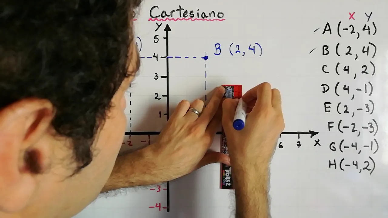
Added:Understanding Cartesian coordinates and plotting discrete data points (x, y).
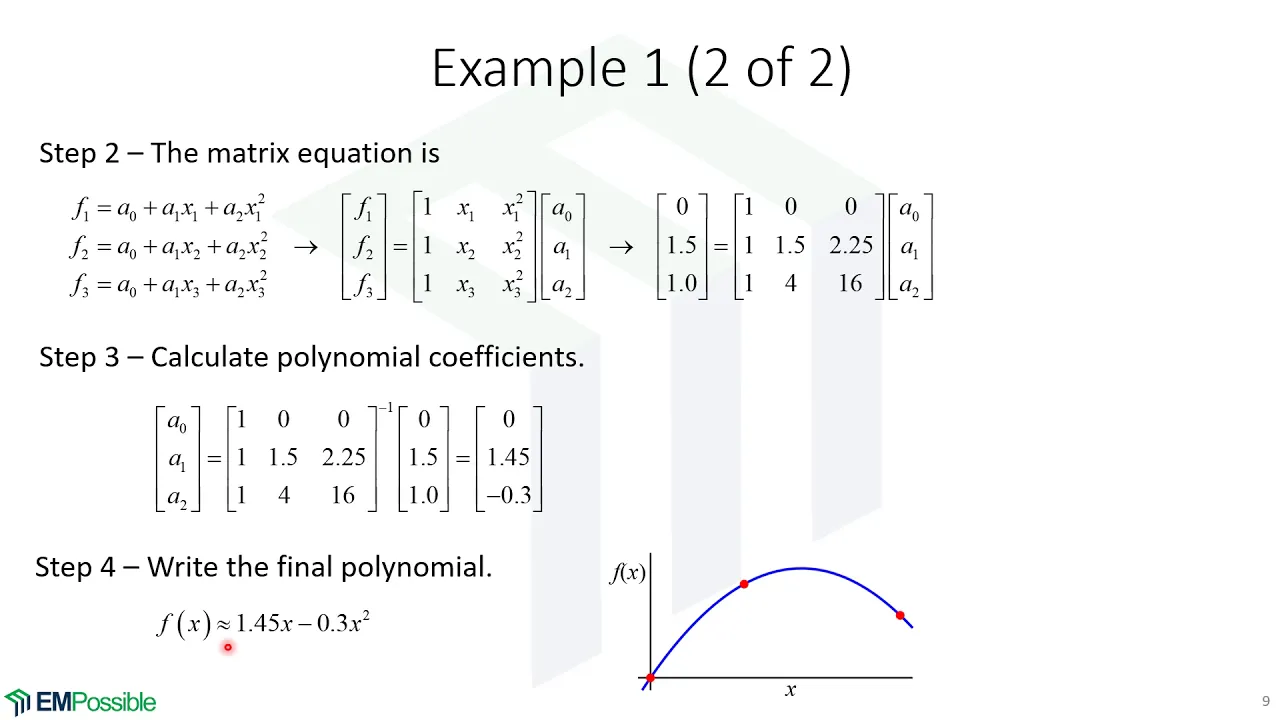
Basic polynomial algebra, including roots of polynomials, expansion, and evaluation.
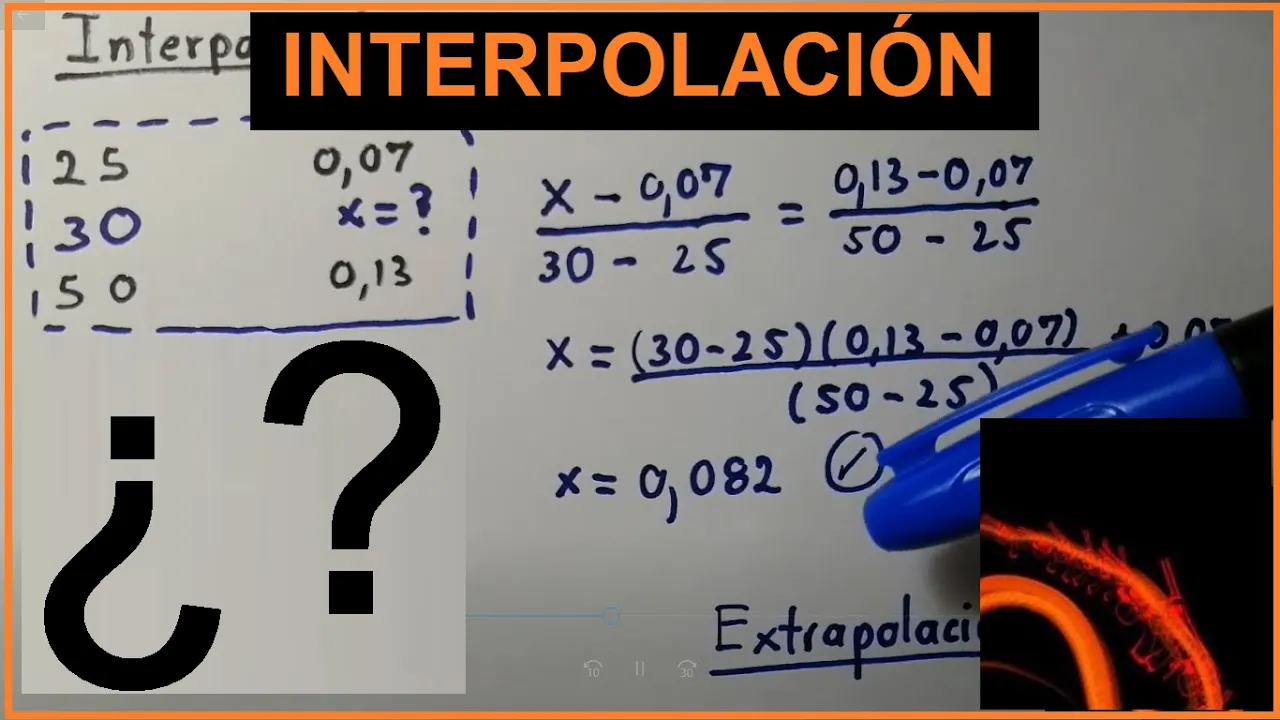
The conceptual difference between interpolation (estimating values within a data range) and extrapolation.
Familiarity with linear interpolation as a baseline for understanding higher-degree polynomial estimation.
Analyzing interpolation error and Runge's phenomenon (oscillations in high-degree polynomials).
Newton's Divided Difference method as a more computationally efficient alternative for dynamic data sets.
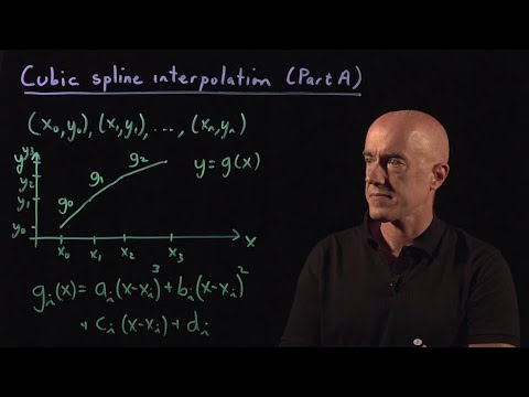
Spline Interpolation (especially Cubic Splines) for smoother, piecewise polynomial curve fitting.
Applying interpolation to numerical calculus, such as formulating Newton-Cotes integration formulas.
330.2K views4.9Klikes8:10Original Release: 2017-06-10
[Music] hey guys welcome back Fred here AF math and Engineering we're going to do a quick question uh quick example for you on how to use uh lrange interpolating polinomial to estimate uh or or fit a polinomial to a set of data you know there's you'll see in the book and in this course there are these really confusing long formulas that a lot of people get kind of thrown off by uh so for this I'm not going to show you the formula I'm just going to show you how I do it and then maybe that can help you understand how to use the formula how to interpret the formula or you can just remember how to do it and not even worry about the formula okay let's just get started and hopefully this is helpful to you okay so let's read the question use lrange interpolating polinomial to estimate F of 2 for the given data okay so what it wants us to do here is it wants us to come up with the The Grange interpolating the polinomial and then plug into and find the final number answer so let's go ahead and begin okay so uh since we have four data sets okay we're going to write F sub3 okay so if we had five uh X1 X 2 X 3 X4 X5 y1 Y 2 1 3 y 4 5 Etc we'd have F of uh sub 4X okay and uh we're going to end up with four terms here okay so the first thing we're going to do okay right off the bat is we're going to look for y1 okay so y1 we're going to start with that we're going to keep that in Brackets okay this gets a little bit long okay so we're going to work down all right so that's the first thing you do go to y1 write it under brackets in here so what we're going to do is is we're going to uh start by writing X okay and each term in uh in the lrange interpolating polinomial in the numerator is going to have this x okay so this x is a variable okay this is don't get this x confused with x sub one x sub 2 okay this is something different so we're going to start with X and we're going to subtract each uh entry in the table here that's not X1 not the one that we're working on okay so remember we went to y1 and we put this one in so X1 and Y now we're not going to include X1 in the numerator in this question okay so uh we're going to start at X2 and we're going to subtract uh X2 from X okay and we're just going to go along and we're going to subtract X3 and we're going to subtract X4 okay there we go easy simple just like that you know no long formulas really straightforward just kind of remember how to do this process so that's for the numerator okay so say we're in this column we're working on this column we're going to say we're going to subtract X from all of these okay and uh the whole thing is Multiplied like I said before by -2 by y1 okay now let's go to the denominator okay so now we're going to take the numerical value of X1 this is where the X1 comes into play which is -2 okay and we're going to subtract that okay by each uh value uh again of the X's that are not X1 okay so minus okay minus one again okay uh - 0 -2 once again so we're subtracting X1 from all of these values here finally we have - 2 - 4 okay simple okay perfect so that is the first term of our lrange polinomial okay and essentially what we're going to do is we're just going to do exactly the same thing for each column okay so we're going to next start at uh Y 2 and then we're going to start at Y3 and y4 so let's just go through them okay and uh all of these are added together by the way so let's start in the next one okay so you get the feel for what this is okay so our Y2 value is four so we're going to multiply four by and then let's draw our line for our fraction okay so now um we're going to we have our variable X and we're going to subtract that by every x value that's not X2 so not that the one that's not in the column of Y2 sorry x - - 2 x - 0 x - 4 okay simple really straightforward okay so nothing to get confused or stressed out over uh just follow these steps next on the denominator okay we're going to look for y uh Y2 the value of x21 so we're going to start at each term with that and we're going to subtract the other X values by this so we have y1 - -2 sorry X2 - X1 okay multiplied by X2 which is -1 - X3 which is 0 and then we have we have X2 -1 - 4 okay super straightforward okay so that's done let's move on to E uh Y3 so starting I'm going to go a little faster now okay let's draw the line for our uh for our fraction here and we go ahead and start with our variable X and we're going to subtract that by all the X's that are not X3 so we're going to start with x - X1 okay x - X2 and X - X4 okay and let's go ahead and do the denominator so we're going to look for the value of x3 which is zero and we're going to just like I said subtract that by all the values of X that are not X3 simple okay so there we have uh x3 - X1 x3 - X2 x3 - X4 finally let's do the last term so just follow this pattern it's the same if you have three value three data points if you have five 6 7 you just follow these steps every time you get 100% simple it's free marks all right let's take a look at this what do we have here we have our variable x uh all the by subtracting by all the values of X in the data points that are not X4 so we're going to start with X1 x - X2 X - X3 okay let's go to the bottom let's start with the value of X4 and then we go X4 4 - X1 X4 - X2 and finally X4 minus X3 and that's it so this here is our lrange interpolate uh lrange polom okay now the the question isn't finish because it asks us to estimate F2 F of two uh and how we do that is pretty simple okay so what we're going to do is now we're going to take our polinomial here and we're going to go ahead and plug in two into X here so that's where that variable X comes into play Okay so let's go ahead and do that so we have F3 of 2 and that is going to be equal to I'm just going to write down the simplified simplified version for you okay so uh what we've done there is we've G A ahead and we plugged in two and uh we've gone ahead and simplified these negatives here and made them positives uh and cleaned it up a little bit and if we go ahead and calculate these four terms we will get -2 - 12.8 + 3 + 1.6 and if we add that up we're going to get -10.2 okay and -10.2 is f of 2 calculated by using the lrange polinomial to estimate F of2 of this given data here okay so essentially what that means is this is a if if you were to plot this on mat lab that would be a kind of like a curve of best fit through these points of data okay and on that curve when X is 2 this is the Y value that's that's what that value means okay so thanks so much for watching guys I hope you learned something there and as always like And subscribe if you enjoyed the video [Music]
Up Next

9:14
Newton Divided Difference Formula | Numerical Methods Full Tutorial
@IclassesForYou
191.2K views•2017-05-19

4:43
Elliptic Curve Cryptography Explained: ECC, ECDSA, ECDH
@PracticalNetworking
28.5K views•2024-10-21

10:44
Fourier Series Introduction: The Big Idea Explained
@DrTrefor
387K views•2021-05-03

6:00
The Mathematical Impossibility of Accurate World Maps
@Vox
23.3M views•2016-12-02
Related Study Plans & Knowledge Roadmaps
Structured learning paths in Mathematics
mathematics
Tensor Calculus: Vectors to Riemann Curvature
01Mathematical Foundations: Linear Algebra & Calculus
02Covectors, Dual Spaces, and Tensor Basics
03The Metric Tensor and Index Gymnastics
+ 2 more learning modules
40h5 modules
Explore Roadmap
mathematics
Gödel's Incompleteness: Logic, Proofs & Limits
01Introduction to Formal Systems & Hilbert's Dream
02Set Theory, Cardinality, and Cantor's Diagonal Argument
03Arithmetization and Gödel Numbering
+ 2 more learning modules
14h5 modules
Explore Roadmap
mathematics
Galois Theory: Fields, Groups & Solvability
01Foundations of Abstract Algebra: Groups & Fields
02Polynomials & Field Extensions
03Splitting Fields & Symmetries
+ 2 more learning modules
24h5 modules
Explore Roadmap
mathematics
Non-Euclidean Geometry: Models & Geodesics
01Euclid's Fifth Postulate and the Birth of New Geometries
02Hyperbolic Space and the Poincaré Disk Model
03Geodesics: Defining Straight Lines in Curved Spaces
+ 2 more learning modules
15h5 modules
Explore Roadmap