Academic Databases
Explore Our Semantic Databases
STEM & Tech
Math, Physics, CS & Engineering...
Economics
Macro, Micro, Econometrics...
Business
Management, Marketing, Finance...
Health & Life Sciences
Biology, Medicine, Neuroscience...
Humanities & Social Sciences
Psychology, Law, Philosophy, History...
General Studies
General & interdisciplinary studies...
Explore Topics
Features

Cubic Spline Interpolation: Natural & Clamped Boundary Conditions

Added: 2026-08-07

Deep Dive

Understanding of basic polynomial interpolation (e.g., Lagrange or Newton) and the limitations of high-degree polynomials, such as Runge's phenomenon.

interpolation polynomial ( première partie)

interpolation polynomial ( première partie)

26.6K

Polynomial interpolation constructs a unique polynomial of degree n that passes through n+1 distinct points (x₀,y₀), (x₁,y₁), ..., (xₙ,yₙ). Three main methods exist: (1) System of equations approach using Vandermonde matrices, (2) Lagrange interpolation formula P(x) = Σ[yᵢ × Lᵢ(x)] where Lᵢ(x) = Π[(x-xⱼ)/(xᵢ-xⱼ)] for j≠i, and (3) Newton's divided differences method using P(x) = f[x₀] + f[x₀,x₁](x-x₀) + ... + f[x₀,...,xₙ](x-x₀)...(x-xₙ₋₁). The error formula E(x) = f⁽ⁿ⁺¹⁾(ξ) × ωₙ₊₁(x)/(n+1)! shows error depends on the (n+1)-th derivative at some unknown ξ. However, Runge's phenomenon demonstrates that increasing interpolation points can actually increase error, particularly near interval edges, as shown with f(x)=1/(1+25x²) on [-1,1]. The optimal solution uses Chebyshev nodes, which are the roots of Chebyshev polynomials Tₙ₊₁(x) = cos((2k-1)π/(2(n+1))) for k=1,...,n+1, distributed more densely near endpoints to minimize maximum error.

Click to watch →

Advanced Mathematics for Engineers Lecture No. 14

Advanced Mathematics for Engineers Lecture No. 14

51.9K

High-degree polynomial interpolation on equally spaced points can produce severe oscillations near interval edges, especially for smooth functions like f(x) = 1/(1+25x²). Adding more points actually increases these oscillations because higher-degree polynomials grow faster (x^20 grows much faster than x^11). This phenomenon, known as Runge's phenomenon, demonstrates why equally spaced points are generally poor choices for interpolation. The fundamental issue is that high-degree polynomials must diverge to infinity as x approaches infinity, creating unavoidable oscillatory behavior.

Click to watch →

Polynomial Interpolation and Runge's Phenomenon | Overview

Polynomial Interpolation and Runge's Phenomenon | Overview

552

Runge's phenomenon reveals a fundamental limitation in polynomial interpolation: increasing the number of interpolation points does not always improve accuracy and may cause severe oscillations at interval endpoints. Using Runge's function f(x) = 1/(1+25x²) as a test case, we observe that high-degree interpolating polynomials constructed with equally spaced points exhibit wild oscillations near -1 and 1, even becoming unrecognizable from the original function. This occurs because two factors combine: higher-order derivatives of smooth functions grow rapidly with degree, and equidistant point placement amplifies these effects through increasing Lebeshev constants. The solution involves using non-equidistant point distributions like Chebyshev nodes, which minimize oscillation and provide more reliable approximations.

Click to watch →

Calculo Numérico (Teoría) 05/09/25

Calculo Numérico (Teoría) 05/09/25

243

This lecture covers numerical polynomial interpolation techniques including Lagrange's method, Newton's divided differences (both progressive and regressive forms), and Newton-Gregory method for equidistant points. The instructor demonstrates how to construct divided differences tables and explains Runge's phenomenon, which shows that increasing polynomial degree with equidistant nodes actually increases error at endpoints. The lecture introduces Chebyshev nodes as an optimal solution that minimizes interpolation error by clustering nodes near interval boundaries, using the formula x_k = cos((2k+1)π/(2n+2)) for normalized interval [-1,1].

Click to watch →

Interpolationspolynom (Lagrange) berechnen | Einfach Erklärt + Vor-&Nachteile

Interpolationspolynom (Lagrange) berechnen | Einfach Erklärt + Vor-&Nachteile

113.4K

The Lagrange interpolation polynomial is a method to construct a polynomial of degree at most n-1 that passes through n given points (x₀,y₀), (x₁,y₁), ..., (xₙ₋₁,yₙ₋₁) by summing the products of each y-value and its corresponding basis function Lᵢ(x), where each basis function Lᵢ(x) is defined as the product of (x - xⱼ)/(xᵢ - xⱼ) for all j ≠ i; this approach offers the advantage of being independent of the y-values when adding new points but suffers from numerical instability and computational inefficiency when the number of points changes.

Click to watch →

Deep Dive

Concepts of continuity (C0) and smoothness/differentiability (C1 and C2) of piecewise functions at knot points.

رياضيات الخامس العلمي 143 / حل تمارين ( 1 - 6 ) صفحة 143 / الفصل السادس

رياضيات الخامس العلمي 143 / حل تمارين ( 1 - 6 ) صفحة 143 / الفصل السادس

149.5K

For piecewise functions, continuity and differentiability must be checked at junction points. Continuity requires three conditions: (1) the function value exists at the point, (2) the left-hand limit equals the right-hand limit, and (3) both limits equal the function value. Differentiability requires the left-hand derivative to equal the right-hand derivative. For f(x) = x² + 1 when x < 2 and f(x) = 7 - x when x ≥ 2, at x = 2: f(2) = 5, left limit = 5, right limit = 5, so it is continuous. However, left-hand derivative = 4 and right-hand derivative = -1, so it is not differentiable. For f(x) = x² when x ≥ -1 and f(x) = -2x - 1 when x < -1, at x = -1: f(-1) = 1, left limit = 1, right limit = 1, so it is continuous. Left-hand derivative = -2 and right-hand derivative = -2, so it is differentiable. For f(x) = x² + 5 when x ≥ 1 and f(x) = ax + b when x < 1, to be differentiable at x = 1: continuity requires a + b = 6, differentiability requires a = 2, so b = 4.

Click to watch →

Continuity & Differentiability in One Shot | JEE ADVANCED 💪 | Concepts + PYQs

Continuity & Differentiability in One Shot | JEE ADVANCED 💪 | Concepts + PYQs

75.9K

For piecewise functions, continuity at boundary points requires left-hand limit equals right-hand limit equals function value. Differentiability requires both left-hand and right-hand derivatives exist and are equal. The instructor demonstrates with f(x) = b1 + cos(πx) for x in [1,2] and f(x) = a1 + sin(πx) for x in [2,3], showing that at x = 2, continuity requires b1 + 1 = a1.

Click to watch →

Funciones a Trozos con UN PUNTO de Ruptura 📉 CONTINUIDAD y DERIVABILIDAD

Funciones a Trozos con UN PUNTO de Ruptura 📉 CONTINUIDAD y DERIVABILIDAD

295.2K

For piecewise functions, continuity requires that the function exists at the rupture point, the limit exists from both sides, and the limit equals the function value; differentiability requires that the left-hand derivative equals the right-hand derivative at the rupture point. If a function is not continuous at a point, it cannot be differentiable there. When a function is continuous but not differentiable at a rupture point, it has a point anguloso (angular point); when it is both continuous and differentiable, it has a punto suave (smooth point).

Click to watch →

الخامس العلمي/ الفصل السادس / المشتقات/ محاضرة 27/ قابلية الاشتقاق

الخامس العلمي/ الفصل السادس / المشتقات/ محاضرة 27/ قابلية الاشتقاق

118.3K

To check continuity of a piecewise function at a boundary point: (1) Calculate the function value at the boundary point, (2) Calculate the right-hand limit, (3) Calculate the left-hand limit, (4) Check if all three values are equal. For f(x) = x² + 1 for x ≥ 2 and f(x) = 7 - x for x < 2: f(2) = 5, right-hand limit = 5, left-hand limit = 5, so it is continuous. For differentiability: (1) Right-hand derivative at x = 2: f(2+h) = (2+h)² + 1 = 5 + 4h + h², [f(2+h) - f(2)]/h = 4 + h, limit is 4. (2) Left-hand derivative: f(2+h) = 7 - (2+h) = 5 - h, [f(2+h) - f(2)]/h = -1, limit is -1. Since 4 ≠ -1, the function is not differentiable at x = 2. A key relationship is that if a function is differentiable at a point, it must be continuous at that point. However, continuity does not imply differentiability.

Click to watch →

رياضيات الخامس العلمي/الفصل السادس/ المحاضرة 5/ تمارين 1-6

رياضيات الخامس العلمي/الفصل السادس/ المحاضرة 5/ تمارين 1-6

223.4K

A function is continuous at a point if the left-hand limit, right-hand limit, and function value all equal the same number. A function is differentiable at a point if the left-hand derivative equals the right-hand derivative. For the piecewise function f(x) = 7 - x when x ≥ 2 and f(x) = x² + 1 when x < 2, at x = 2: f(2) = 5, left limit = 5, right limit = 5, so it is continuous. However, f'(2⁺) = -1 and f'(2⁻) = 4, so it is not differentiable. For f(x) = x² when x ≥ -1 and f(x) = -x - 1 when x < -1, at x = -1: f(-1) = 1, left limit = 1, right limit = 1, so it is continuous. The right-hand derivative f'(-1⁺) = -2, but the left-hand derivative does not exist, so it is not differentiable.

Click to watch →

Deep Dive

Solid grounding in introductory calculus, specifically computing first and second derivatives of polynomial equations.

1st and 2nd Derivative of a Polynomial | Calculus

1st and 2nd Derivative of a Polynomial | Calculus

138

To find the first derivative of a polynomial function, apply the power rule to each term by bringing down the exponent as a coefficient, multiplying it by the existing coefficient, and reducing the exponent by one; the derivative of a constant is zero. To find the second derivative, repeat the process on the first derivative. Evaluating the first derivative at a point reveals whether the original function is increasing (positive value) or decreasing (negative value) at that location. Evaluating the second derivative at a point indicates the concavity of the original function: a positive value means the function is concave up, while a negative value means it is concave down.

Click to watch →

Differential Calculus: ch2.1 #4 / AP Calculus: ch2.1 #4

Differential Calculus: ch2.1 #4 / AP Calculus: ch2.1 #4

585

To find the first and second derivatives of a polynomial function, first expand the expression, then apply the power rule (d/dx of x^n = n*x^(n-1)) to each term, and finally differentiate again for the second derivative; for polynomial functions, the domain is all real numbers since there are no denominators or restricted functions.

Click to watch →

ejemploCriterioSegundaDerivada

ejemploCriterioSegundaDerivada

231

For the function f(x) = x³ + 3x² - 2, the first derivative is f'(x) = 3x² + 6x, and the second derivative is f''(x) = 6x + 6. The derivative of a constant term is zero, and the power rule states that the derivative of xⁿ is n·xⁿ⁻¹.

Click to watch →

Exercise 2.7 |12th Math |Successive Derivatives |

Exercise 2.7 |12th Math |Successive Derivatives |

333

For polynomial functions, apply the power rule to each term. For y = x⁵ - 3x⁴ + 4x³ + x - 2, y1 = 5x⁴ - 12x³ + 12x² + 1, and y2 = 20x³ - 36x² + 24x. Constants become zero, and each term's power decreases by 1 while the original power becomes the coefficient.

Click to watch →

Les fonctions à plusieurs variables (extremums)

Les fonctions à plusieurs variables (extremums)

1.8K

This segment teaches how to calculate first and second derivatives of polynomial functions. The instructor demonstrates finding the first derivative of f(x) = x³ - x², which yields f'(x) = 3x² - 2x. The second derivative is then calculated as f''(x) = 6x - 2. The process involves applying differentiation rules to each term of the polynomial, reducing the power by one and multiplying by the original power. This foundational skill is essential for analyzing function behavior and finding critical points.

Click to watch →

Deep Dive

Proficiency in linear algebra, particularly representing and solving systems of linear equations using matrices (e.g., tridiagonal matrices).

Che cos'è l'algebra lineare? Che cosa studia?

Che cos'è l'algebra lineare? Che cosa studia?

8.9K

Linear transformations can be represented as matrices (rectangular arrays of numbers). For example, F(x,y,z) = 4x + 7y + 8z becomes the matrix [4, 7, 8] acting on vector [x, y, z]ᵀ. Matrices also represent systems of linear equations: [4, 7, 8; 9, 8, 5; 10, -4, 8] × [x, y, z]ᵀ = [10, 7, 4]ᵀ. This representation enables systematic solving using methods like Gaussian elimination. Matrices provide a powerful framework for studying linear transformations and solving linear systems.

Click to watch →

CLASE 9 NUMERICOS

CLASE 9 NUMERICOS

129

The Thomas algorithm (tridiagonal matrix algorithm) efficiently solves systems with tridiagonal matrices (non-zero elements only on the main diagonal and adjacent diagonals). It decomposes the matrix into L and U matrices with specific structure. The forward elimination modifies the system by computing modified E and F values: E_k = E_k / F_{k-1}, F_k = F_k - E_k * G_{k-1}. The backward substitution then solves the modified system. This method runs in O(n) time, much faster than general Gaussian elimination. The L matrix has 1s on the diagonal and modified E values on the subdiagonal, while U has modified F values on the diagonal and modified E values on the superdiagonal.

Click to watch →

Lec 1 | MIT 18.085 Computational Science and Engineering I, Fall 2008

Lec 1 | MIT 18.085 Computational Science and Engineering I, Fall 2008

441.1K

A tridiagonal matrix is a sparse matrix with non-zero elements only on the main diagonal and the two adjacent diagonals (one above and one below). These matrices arise frequently in numerical methods, particularly from discretizations of second-order differential equations. The tridiagonal structure significantly reduces computational complexity when solving systems of equations.

Click to watch →

📈 مكثف الجبر الخطي – تشابتر ون بدون تعقيد | Linear Algebra Chapter 1

📈 مكثف الجبر الخطي – تشابتر ون بدون تعقيد | Linear Algebra Chapter 1

4.6K

A linear system Ax = b can be represented using three matrices: (1) Coefficient matrix A (contains coefficients of variables), (2) Variable matrix x (contains variables), (3) Constant matrix b (contains equation results). This representation allows solving systems using matrix operations.

Click to watch →

Tridiagonal Matrix for Linear Equations

Tridiagonal Matrix for Linear Equations

527

The Thomas Algorithm is an efficient O(n) method for solving tridiagonal matrix systems, which are square matrices with non-zero elements only on the main diagonal and the adjacent super/sub-diagonals; the algorithm proceeds through three phases: forward elimination to compute alpha values (α₁ = B₁, αᵢ = Bᵢ - Aᵢ×Cᵢ₋₁/αᵢ₋₁), backward substitution to compute beta values (β₁ = D₁/B₁, βᵢ = (Dᵢ - Aᵢ×βᵢ₋₁)/αᵢ), and final solution computation (xₙ = βₙ, xᵢ = βᵢ - Cᵢ×xᵢ₊₁/αᵢ).

Click to watch →

Setup & Equations

Deriving Equations

Matching Conditions

Boundary Conditions

System Solution

Final Natural Spline

Clamped Spline Setup

Clamped System Solve

Compare Results

Setup & Equations

0:03

Playing Section

1
Define two polynomial regions for three data points.
2
Establish general cubic spline forms for each interval.
3
Identify eight unknown coefficients to be solved.

Deep Dive

Exploration of alternative boundary conditions, such as 'not-a-knot', periodic, or Hermite boundary conditions.

Ch03n2: Other Types of Boundary Conditions for Cubic Splines

Ch03n2: Other Types of Boundary Conditions for Cubic Splines

4.2K

This video explains two alternative boundary conditions for cubic splines beyond the natural cubic spline: (1) Not-a-knot condition, which requires the two polynomials at each endpoint to be identical (s₀ = s₁ and sₙ₋₂ = sₙ₋₁), providing fourth-order approximation accuracy; and (2) Periodic boundary conditions, which enforce periodic behavior by requiring the spline values, first derivatives, and second derivatives to match at the endpoints (Z₀ = Zₙ), making them suitable for modeling periodic physical phenomena. Both conditions modify the linear system of equations used to solve for the second derivatives (Z_i), with the coefficient matrix becoming almost tri-diagonal rather than fully tri-diagonal.

Click to watch →

09: Clenshaw-Algorithmus, Splines, Kubische Splines

09: Clenshaw-Algorithmus, Splines, Kubische Splines

8K

Three types of boundary conditions define different classes of splines: (1) Clamped/Clamped spline: the first derivatives at both ends are specified (prescribed slopes), (2) Natural spline: the second derivatives at both ends are zero (free ends), and (3) Periodic spline: the function and its first and second derivatives match at the endpoints (periodic extension). Each type provides two additional equations needed to solve the system of equations for the spline coefficients.

Click to watch →

Kubische Spline Interpolation, Numerische Methoden #17

Kubische Spline Interpolation, Numerische Methoden #17

423

Three types of boundary conditions exist for cubic splines: (1) Natural boundary conditions require the second derivative to be zero at both endpoints; (2) Clamped (or Hermite) boundary conditions specify prescribed first derivatives at the endpoints; (3) Periodic boundary conditions require that the function values and both derivatives match at the endpoints, allowing the spline to be extended periodically.

Click to watch →

Advanced Mathematics for Engineers Lecture No. 15

Advanced Mathematics for Engineers Lecture No. 15

3.7K

Natural splines (y''=0 at boundaries) are one choice. Alternatives include: specifying second derivatives at boundaries, requiring constant curvature at boundaries, or specifying first derivatives at boundaries. For periodic functions, the spline must satisfy: s'(x₀) = s'(xₙ) and s''(x₀) = s''(xₙ). Additionally, the data must satisfy y₀ = yₙ for continuity. These conditions ensure the spline repeats smoothly when extended periodically.

Click to watch →

Интерполяция с кратными узлами, сплайнами. Кубический сплайн. Среднеквадратичное приближение. Лек. 6

Интерполяция с кратными узлами, сплайнами. Кубический сплайн. Среднеквадратичное приближение. Лек. 6

671

A cubic spline S(x) on [a,b] with nodes x_0,...,x_n satisfies: (1) S(x) is a cubic polynomial on each interval [x_i, x_{i+1}], (2) S, S', S'' are continuous at all nodes, (3) S(x_i) = f(x_i) for all i. Boundary conditions are needed to uniquely determine the spline. Natural boundary conditions set S''(x_0) = S''(x_n) = 0. Alternative conditions include clamped (first derivative specified) or periodic (S(a) = S(b), S'(a) = S'(b)).

Click to watch →

Deep Dive

Introduction to B-Splines (Basis Splines) and NURBS (Non-Uniform Rational B-Splines) for advanced curve design in computer graphics and CAD.

Lec-47 B-Spline Curve

Lec-47 B-Spline Curve

127.1K

B-spline curves offer significant advantages over Bezier curves by allowing independent specification of curve order (k) from the number of control points, enabling local propagation where changing a control point affects only nearby segments rather than the entire curve. The curve is composed of n-k+2 segments with C^(k-2) continuity, where k=3 provides slope continuity and k=4 provides curvature continuity. NURBS (Non-Uniform Rational B-splines) extend B-splines by introducing weights to control points, enabling exact representation of conic sections like circles, ellipses, parabolas, and hyperbolas, which cannot be achieved with standard B-splines or Bezier curves. This mathematical flexibility makes NURBS the industry standard for representing curves and surfaces in computer-aided design.

Click to watch →

B-Splines

B-Splines

121.2K

B-Splines (basis splines) are piecewise polynomial curves formed by joining multiple Bezier curves together, where a k-degree B-Spline with n+1 control points consists of n-k+1 Bezier curves that meet with C² continuity (matching position, first derivative, and second derivative at junctions); unlike Bezier curves which have degree equal to the number of control points minus one, B-Splines allow many control points to define a single smooth curve of lower degree, making them more flexible for complex shapes while maintaining computational efficiency.

Click to watch →

B-Spline & NURBS Theory

B-Spline & NURBS Theory

2.7K

B-Spline curves overcome the limitations of basic Bezier curves by introducing an order parameter (K) that separates the curve's degree from the number of control points, enabling local control where each control point influences only specific curve segments rather than the entire curve; the number of segments equals n-K+2, the maximum degree is K-1, and continuity is K-2, while NURBS (Non-Uniform Rational B-Splines) further extends this capability by incorporating weightage factors (wi) that allow the curve to pass through specific control points and can represent any analytical curve including conic sections.

Click to watch →

B-Splines

B-Splines

45.2K

B-Splines (Basis Splines) address the computational limitations of high-degree Bezier curves by combining multiple low-degree Bezier segments. A k-degree B-Spline with n+1 control points consists of n-k+1 Bezier curves joined end-to-end. The method satisfies C0, C1, and C2 continuity conditions to ensure smooth, gap-free curves without abrupt directional changes. Like Bezier curves, B-Splines are defined as weighted sums of basis functions multiplied by control points, where the basis functions determine which control points influence each curve segment.

Click to watch →

Non uniform rational B Spline curve - Introduction to Computer Graphics and Output Primitives

Non uniform rational B Spline curve - Introduction to Computer Graphics and Output Primitives

1.4K

A Non-uniform Rational B-Spline (NURBS) curve is a mathematical representation in computer graphics that extends B-spline curves by incorporating weighted control points, enabling the curve to pass through specified points by adjusting weights and allowing representation of complex shapes including conic sections like circles; unlike standard B-splines where the curve doesn't necessarily pass through control points, NURBS provides local control over curve segments and maintains the smoothness properties of B-splines while offering greater flexibility in geometric modeling.

Click to watch →

Deep Dive

Implementation of spline interpolation algorithms in programming environments (e.g., Python with SciPy, MATLAB, or R) for data smoothing and curve fitting.

Spline Interpolation In Python (Linear, Quadratic, Cubic, etc…) | Numerical Methods

Spline Interpolation In Python (Linear, Quadratic, Cubic, etc…) | Numerical Methods

20.4K

This comprehensive section covers three spline interpolation techniques in Python. First, generate evenly spaced x-values using numpy.linspace between your data's min and max. For linear interpolation, use scipy.interpolate.interp1d with kind='linear' to create an interpolation function. For quadratic interpolation, set kind='quadratic'—note that insufficient x-intervals may produce visually angular results. For cubic interpolation, set kind='cubic', though this basic form lacks boundary condition control. For advanced cubic spline with boundary conditions, use scipy.interpolate.CubicSpline and specify conditions like 'natural' (zero second derivative at endpoints) for more appropriate fitting behavior.

Click to watch →

Spline Interpolation Example with SciPy

Spline Interpolation Example with SciPy

1.4K

Spline interpolation is a piecewise polynomial interpolation technique that creates smooth curves passing through given data points by dividing intervals into subintervals and fitting polynomials that connect smoothly at these points; in Python, this can be implemented using SciPy's splrep() function to obtain B-spline coefficients and splev() function to evaluate the interpolated values, offering a more flexible alternative to linear interpolation which only connects points with straight lines.

Click to watch →

COSC370 - Interpolation and Curve Fitting (Part 3)

COSC370 - Interpolation and Curve Fitting (Part 3)

502

A Python implementation of cubic spline interpolation consists of two main functions: (1) a function to compute the curvatures by solving the tridiagonal linear system, and (2) a function to evaluate the spline at any point by determining which subinterval the point lies in and applying the appropriate cubic polynomial. The implementation uses numpy for array operations and matrix decomposition (LU decomposition) to solve the linear system efficiently. The spline evaluation requires identifying the correct subinterval and applying the cubic formula with the computed curvatures.

Click to watch →

5.2.7-Curve Fitting: Spline Interpolation

5.2.7-Curve Fitting: Spline Interpolation

115.9K

Spline interpolation provides a superior alternative to polynomial interpolation by using piecewise polynomial functions (linear, quadratic, or cubic) that pass through given data points while maintaining smoothness. Linear splines connect points with straight lines but have discontinuous first derivatives at knots. Quadratic splines ensure both function value and first derivative continuity at interior knots, requiring the second derivative to be zero at the first point for constraint. Cubic splines further enforce second derivative continuity at all interior knots, producing the smoothest approximation that avoids overfitting while accurately representing the underlying function.

Click to watch →

CHEN 6400: lecture 8 - Interpolation, regression, integration

CHEN 6400: lecture 8 - Interpolation, regression, integration

132

High-order polynomial interpolation (>3rd order) causes oscillation and unphysical behavior at boundaries. Cubic splines solve this by fitting separate cubic polynomials between each data point pair while ensuring smoothness. Each cubic has four coefficients requiring boundary conditions on slopes and derivatives. Python's scipy.interpolate.CubicSpline implements this by storing cubic polynomials between every point pair. The method provides stable, smooth interpolation without oscillation or unbounded values. Implementation involves importing CubicSpline, creating an instance with x and y data, then evaluating at desired points.

Click to watch →

Deep Dive

Multidimensional interpolation techniques, such as bicubic spline interpolation used in digital image processing and geospatial modeling.

lecture 13 - Interpolation Part 2

lecture 13 - Interpolation Part 2

172

Multi-dimensional interpolation extends to multiple independent variables (e.g., pressure as a function of temperature and density). The simplest robust method is linear interpolation in each dimension sequentially. For example, with a 2D table, first interpolate in one direction, then interpolate the results in the other direction. This breaks down complex multi-dimensional problems into multiple 1D interpolation steps, though complexity increases exponentially with dimensions.

Click to watch →

Multivariate interpolation

Multivariate interpolation

1.8K

Multivariate interpolation is a numerical analysis technique for estimating function values at arbitrary points when the function is known only at discrete locations, with applications ranging from geostatistical digital elevation modeling to image processing; common methods include nearest neighbor, bilinear/bicubic interpolation, Delaunay triangulation, inverse distance weighting, radial basis functions, and spline interpolation, which can be generalized to any number of dimensions using tensor product constructions.

Click to watch →

Image interpolation(nearest neighbour interpolation,bilinear and bicubic interpolation).

Image interpolation(nearest neighbour interpolation,bilinear and bicubic interpolation).

16.6K

Image interpolation is a technique for estimating unknown pixel values when resizing or transforming images, with three main methods: nearest neighbor interpolation assigns new pixels the same value as their closest existing neighbor (fastest but causes pixelation), bilinear interpolation calculates a weighted average of the four nearest neighboring pixels (provides smoother results but may blur edges), and bicubic interpolation uses a cubic polynomial fitted to 16 surrounding pixels (offers the smoothest results but requires more computation); the choice of method depends on the image's complexity and available computational resources.

Click to watch →

Bicubic Interpolation - Computerphile

Bicubic Interpolation - Computerphile

274.8K

Bicubic interpolation is an advanced image scaling technique that estimates new pixel values by considering a larger neighborhood of surrounding pixels (typically 4x4 grid) compared to simpler methods like nearest neighbor or bilinear interpolation, resulting in smoother and more visually accurate image resizing by calculating weighted averages based on cubic polynomial functions.

Click to watch →

Raster Interpolation Explained

Raster Interpolation Explained

778

Raster interpolation computes pixel values at specific locations and scales through three primary methods: nearest neighbor (assigns constant values across cells with sharp edges), bilinear interpolation (linear averaging between four surrounding cells without overshoot/undershoot), and bicubic interpolation (smooth cubic spline using 16 surrounding cells which may return values outside the original data range). These methods are applied during rendering, overview generation, virtual raster creation, and point inspection, with method selection dependent on field type (continuous, image, classified, or image palette) and band data type (decimal or integer). Key pitfalls include cubic interpolation causing overflow/underflow (values exceeding source range) and ringing artifacts near abrupt slope changes, while edge effects differ between interpolation methods.

Click to watch →

Setup & Equations

Deriving Equations

Matching Conditions

Boundary Conditions

System Solution

Final Natural Spline

Clamped Spline Setup

Clamped System Solve

Compare Results

Setup & Equations

0:03

Playing Section

1
Define two polynomial regions for three data points.
2
Establish general cubic spline forms for each interval.
3
Identify eight unknown coefficients to be solved.

258.1K views2.1K18:07@the-Math-guyOriginal Release: 2017-10-30

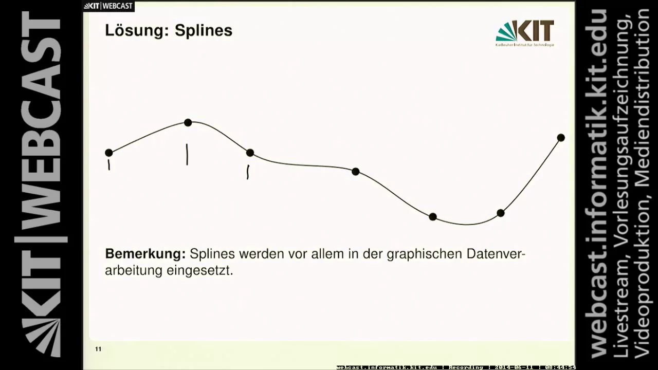
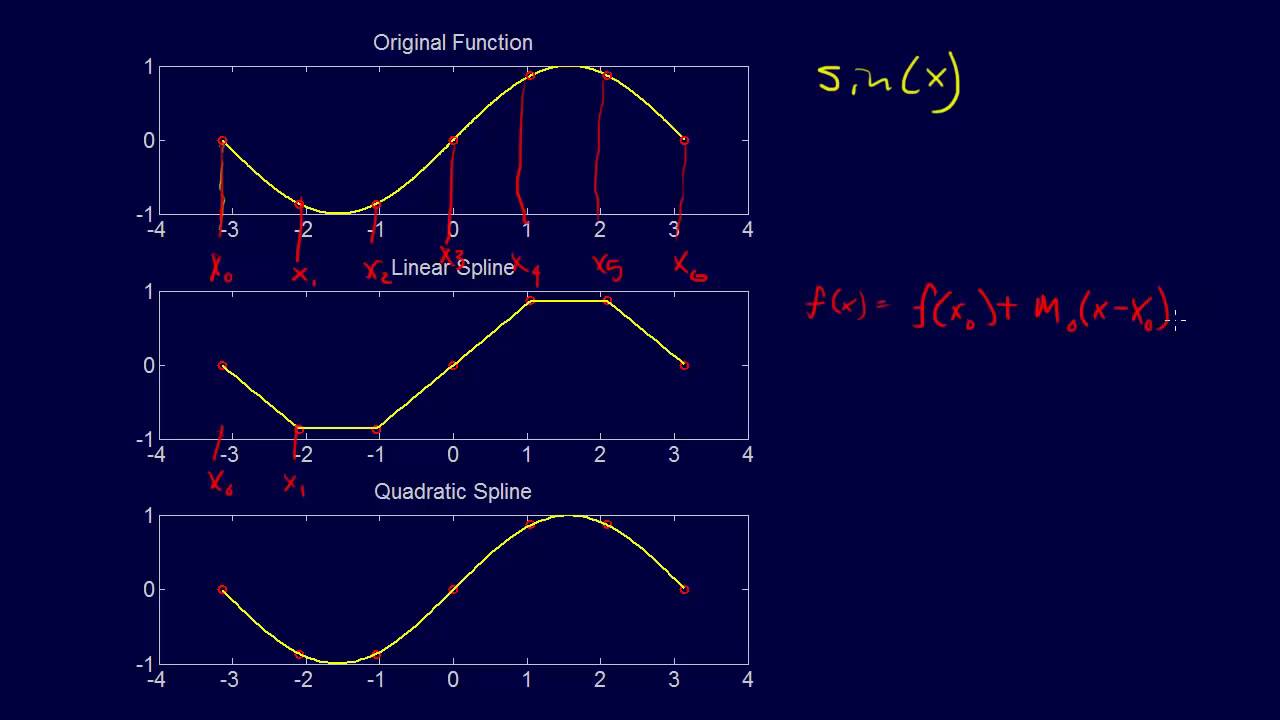
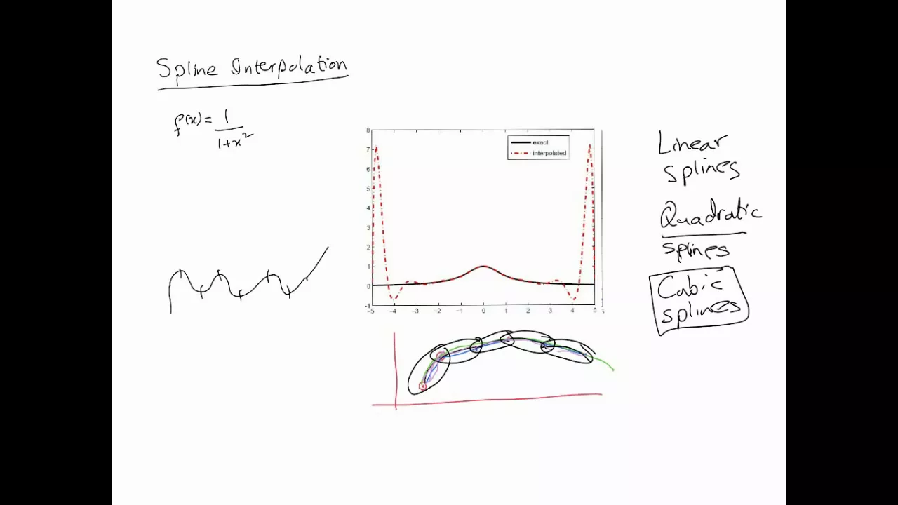
Cubic spline interpolation constructs smooth piecewise polynomials passing through given data points by solving a system of equations derived from point matching, continuity of first and second derivatives at interior points, and boundary conditions. In natural cubic spline, the boundary conditions set the second derivatives at endpoints to zero, while clamped cubic spline uses specified first derivative values at endpoints. For three data points (1,2), (2,3), and (3,5), the natural cubic spline yields polynomials: s₀(x) = 2 + (3/4)(x-1) + (1/4)(x-1)³ for [1,2], and s₁(x) = 3 + (3/2)(x-2) + (3/4)(x-2)² - (1/4)(x-2)³ for [2,3]. With clamped conditions s'(1)=2 and s'(3)=1, the coefficients change accordingly, demonstrating how different boundary conditions produce distinct spline solutions.

[00:00:03]so there are this in this video I'm going to look at cubic spline examples so the question is constructive natural cubic spline that passes through the points 1 2 to 3 & 3 5 now there are two regions here the number X our X points data points belong to one two okay and the other one is of course 2 2 3 okay so within 1 2 we have the polynomial as 0 of X equal so we have that and you'll see that this point here this number here 1 X minus 1 squared X minus 1 sorry X minus 1 X minus 1 squared and cubed this one comes from this the first point in the interval so so now the next one is of course s 1 of X and that's equal to a1 plus b1 into similarly the first point in this is 2 here so this will be X minus 2 this second polynomial so your first step will always be split the regions and for each region you see here there will be a polynomial so there's two polynomials in this case three points means there will be two polynomials two splines so next we our next objective is going to be to look for these eight these eight unknowns so we have eight unknowns to find eight unknowns to find eight unknowns to start with we'll use the point 1/2 so s 0 of 1 should be equal to 2 which means as we substitute the point 1 into S 0 you will see here that this will go to 0 this will go to 0 and this will go to 0 and all it'll leave is the a 0 so a 0 equals 2 so we have one of the points and so we have seven more to go so he found one of these ok similarly we'll go to the next point so s 0 of 2 in fact is equal to so now we have to let me just clarify something here you see these two points here 1 2 & 2 3 ok both are both are in this region from 1 to 2 ok and these two points well this is an overlap and this point are both in this other region 2 3 so the 2 3 point here this one here that you see is overlapping this is where the matching condition also will apply so anyway as 0 of 2 should be 3 according to the data so that means we'll end up with so what's going on here just to show you so what I've done is basically I'm substituting this 2 into here so 2 minus 1 2 minus 1 2 minus 1 all these are ones so you end up with a 0 plus B 0 C 0 D 0 now a 0 we already have so I'm gonna replace that ok and I'm gonna put in sorry this one second I'm gonna put in instead of a 0 will substitute the 2 but anyway this should be equal to 3 and this implies that we end up so we end up with B 0 plus C 0 plus D 0 equals 1 because put in the the value of a 0 is 2 so we end up with this and we label this as equation 1 now we'll go to the next one which is in the second polynomial so let's use the other two data points so we'll use now s 1 of 2 and that's equal to 3 as well remember that also is the matching condition so s 1 of 2 means that when we substitute that end we end up with a 1 equals 3 because when the 2 goes in this will be 0 0 and 0 so they'll all disappear just leave this a 1 alone so a 1 should be equal to 3 so let's put a box around that now we have in fact 6 unknowns to find still and so far we've got one equation so let's move further on as one of the other and last point now is 3 and it should be equal to 5 and s 1 of 3 equals 5 means when we substitute that in we end up with so we'll end up with this does it take the 3 across the other side so we end up with this equation B 1 plus C 1 plus D 1 equals a 2 so we labeled that as our second equation now we'll start using now we'll start using the matching second matching condition which is on the first derivative so let's do that so s 0 dash of X let's compute that as 0 dash of x is going to be a sorry so the first derivative of s 0 turns out to be this B 0 plus 2 0 0 into X minus 1 plus 3 D 0 and X minus 1 squared similarly s 1 prime turns out to be turns out to be this ok so let's move on so the matching addition s 0 dash of 2 should equal s 1 dash of 2 this implies that we will have the situation when we substitute the 2 into the first one here the 0 derivative we end up with B 0 plus 2 0 0 plus 3 D 0 and that should be equal to when we substitute the 2 into the second this equation that you see here the S 1 Prime everything turns to 0 except B 1 so we have this and this turns out to be the equation so we'll label this as equation 3 the other matching condition remember is as same thing only with the second derivative now in order to do that let's just this this implies of course that the second derivative of s 0 turns out to be - c0 + 6 D 0 into X minus 1 ok and this one s 1 double prime of X turns out to be of course 2 c1 + 6 D 1 into X - 2 so now when we substitute and into the first of these the number 2 for X we end up with this implies that we get to C 0 okay + 6 D 0 equals and then the other one we'll put the 2 in remember so that will give us equals to C 1 so that is equation 4 alright now let's move on now now we all applied all the matching conditions so now the only thing that remains is to apply the boundary condition so the boundary condition the boundary condition B see here just short s 0 double prime of the first of the end one of the endpoints the starting point which is 1 should be equal to 0 and of course the other one will be that I'm sorry s one because the other point is 3 remember the other end point so that will that is for this polynomial s 1 double prime of 3 and that should be also equal to 0 so these are the boundary conditions now these conditions will imply the first one of these implies that s 1 double prime s 0 double prime of 1 so if I substitute the 1 in here you'll see that'll go away and leave you with the 2 C 0 so that means that C 0 equals 0 so we found yet another one of the unknowns so we still have now now we've got five to go ok five to go anyway this condition here implies that in the second this expression here the second derivative we put in 3 instead of X so 3 minus 2 is 1 so 2 c1 2 c1 + 6 D 1 equals 0 and we label this as equation 5 so if you see now we've got 5 and we've got five equations now let's update and collect these together with the value of c0 also updating the equations and let's summarize the equations below or next sorry let's summarize the equations next so this is the summary of the equations as you can see here we've got the five equations and we've got five unknowns now I'll I'm not gonna show you the whole solution but I can show you how you can proceed and the one way to do this is of course the best way to do this is to go by solving this as a system of linear equations and that means you need to order your your unknowns first and the order we we we have here is as follows so we have basically got this order B 0 D 0 ok and then B 1 C 1 D 1 and our right hand side so accordingly we'll end up with this system let me just show you here quickly so you have 1 1 and then 0 0 0 the first equation and then 1 and the second equation will be 0 0 1 1 1 2 and then the third equation will be 1 3 D 0 D 0 and minus B 1 minus B 1 so minus 1 0 0 0 this equation here so that's this one done this one done this one done this will be 3 D 0 minus C 1 so 0 3 and the last one will be wait wait excuse me sorry sorry sorry sorry yeah no it's okay right let's finish this off so the last one which is this 1 2 C 1 so 0 B 0 ok 0 and then 0 here as well 2 6 0 so there you have your Augmented matrix and you can use something as simple as Gaussian elimination to solve this and when you do we get this result this implies that B 0 it turns out to be equal to 3 over 4 ok and D 0 is gonna be 1/4 ok and B 1 B 1 is 3 over 2 and then we have C 1 so C 1 is going to be 3 over 4 and D 1 last one here is going to be minus 1/4 so these are these are the values now how we write the final is as follows so we have 2 so this will be the first polynomial remember now let me bring back here remember a is 0 we already have these so just to remind you let's go back here there's a 0 is 2 and a 1 is 3 and remember C 0 is 0 ok so a 0 2 & 3 so a 0 is 2 so a 0 is 2 a 1 is 3 and C 0 is 0 so now we've got one two three four five six and eight of our unknowns so now as we put these together remember the first polynomial is the the with the zero subscript so a 0 is 2 B 0 is 3 over 4 so plus 3 over 4 into X minus 1 okay and then C 0 is 0 so nothing there and D 0 is a so you'll get plus a quarter into X minus 1 cubed and this is for of course X in the first region or the first range first region yeah 1 2 and then the next polynomial is going to be the though the subscript ones so a 1 a 1 is 3 plus B 1 is 3 over 2 into X minus 2 plus C 1 is 3 over 4 into X minus 2 squared plus D 1 is negative 1/4 into X minus 2 cubed and this is for X in the region 2 2 3 so that is that completes our cubic spline interpolation for the three data points so just as an added example just to show you that we used the natural we found the natural cubic spline in this example which you see above there now if we want to do the same problem but find the clamped cubic spline remember all the conditions will be the same except let me just go back here very quickly and you saw this condition here this is the condition that will change everything above all of these conditions and everything all of the equations everything is fine up to equation up to this equation up to 4 everything's good but this these two conditions now will be replaced by other conditions so if we were to do that let's let's so therefore look at trying to continue this with with these two conditions changed and let's see what happens so let's see what happens so let's do that let me just say something else here important in order to solve this problem first of all you will have to be given this condition that s 1 - that s dash of 1 is equal to 2 and s dash at the other endpoint 3 is equal to 1 so these have to be given to you in the question okay so given these conditions this means that s0 - of one should be - and of course s 1 - of 3 should be equal to 1 so these are the two additional conditions and then when we apply these conditions to our polynomial if we go back here I see here this is where we are now this is our s 0 and s 1 this is this is here you'll see as 0 - is this one and s 1 - is this one so we are applying s 0 - of 1 which means all of these will disappear and leave you just with the be 0 here ok so that will mean that B 0 is 2 and s 1 prime of 3 is gonna give us an equation so let's have a look and what results so let's just do that and if if we do we end up with this condition tells us that clearly B 0 is equal to 2 and s 1 3 - is equal to 3 gives us this equation that be easier be sorry 1 plus 2 C 1 + 3 D 1 is equal to 1 so we get this equation so now if we were to summarize our equations I've just written them here again for you a 0 is 2 so all of these equations now we need to update them with B 0 equals 2 so if we do that in here so if I can so this equation this will be changed and this will become C 0 plus D 0 equals the B 0 is to go the other side gives us minus 1 ok and this equation of course will also need to be updated and will be 2 C 0 + 3 D 0 minus B 1 equals we'll take the 2 to the other side so it's minus 2 so that becomes minus 2 so that one's updated and now we have this system of equations which when we solve in fact like I said in the previous in the previous example as we solve it to be end up with the following result s of X turns out to be this time equal to you can see here this is the resulting polynomial and what I want to do is just show you both here so you can see the difference between these two here you'll see that 2 3 same 2 3 same three 4s changed as you can see this is 2 this this 3 over 2 is the same this 1/4 has become minus 5 over 2 it's this is different as well and you can see there's a cubic appearing here and there was there here the square was missing now it's appearing here and so on so anyway you can see the clamped condition gives you a different polynomial fit or a cubic spline so now this brings us to the end of this example so we've looked at two examples one with the same same three data points nor natural cubic spline and clamped cubic splines we'll stop

Up Next

Simpson's Rule & Numerical Integration | Calculus Tutorial

@TheOrganicChemistryTutor

812.9K views•2018-03-13

Gain Recalibration in Hippocampal Path Integration: Math Theory

@1024kyz

144 views•2020-07-02

Cubic Spline Interpolation Basics | Numerical Analysis

@the-Math-guy

88.6K views•2017-10-30

The Mathematical Impossibility of Accurate World Maps

@Vox

23.3M views•2016-12-02

Related Study Plans & Knowledge Roadmaps

Structured learning paths in Mathematics

View All Mathematics Topics

Non-Euclidean Geometry: Models & Geodesics

01Euclid's Fifth Postulate and the Birth of New Geometries

02Hyperbolic Space and the Poincaré Disk Model

03Geodesics: Defining Straight Lines in Curved Spaces

+ 2 more learning modules

Explore Roadmap

Knot Theory — Moves, Coloring & Polynomials

01Introduction to Topology and Knots

02Reidemeister Moves & Knot Equivalence

03Knot Invariants and Tricolorability

+ 2 more learning modules

Explore Roadmap

Category Theory: Functors, Monads & FP

01Mathematical Foundations: Functions, Composition & Types

02Introduction to Category Theory: Objects & Morphisms

03Functors: Mapping Between Categories

+ 2 more learning modules

Explore Roadmap

Complex Analysis: Residues & Contour Integrals

01Foundations of Complex Numbers

02Complex Functions and Holomorphic Properties

03Complex Integration and Cauchy's Theorem

+ 2 more learning modules

Explore Roadmap