![[PPT] Đa Thức Nội Suy Largrange & Newton](https://i.ytimg.com/vi/aMSw8MV47ds/maxresdefault.jpg)
![[UT#26] Construction des polynômes interpolateurs de Lagrange](https://i.ytimg.com/vi_webp/kY_xA4qw5l8/maxresdefault.webp)















![[W10-4] smoothing spline](https://i.ytimg.com/vi_webp/jPSAX2W0MEI/maxresdefault.webp)
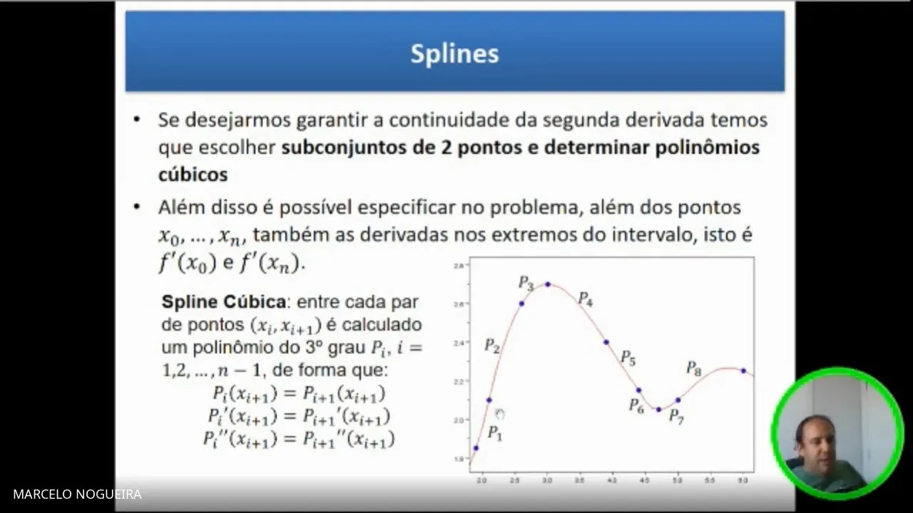
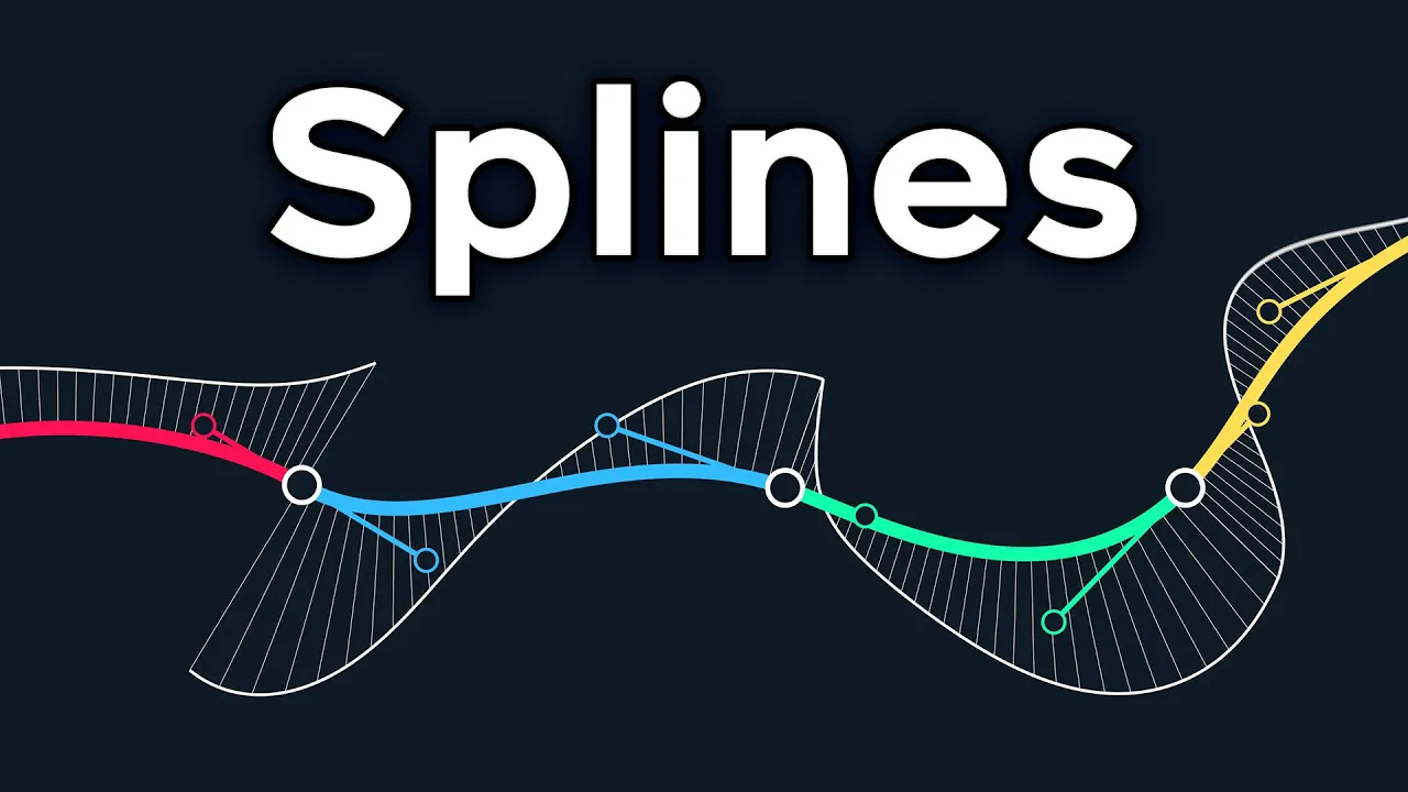
Cubic spline interpolation is a numerical method that addresses the limitations of high-order polynomial interpolation by dividing the interpolation interval into smaller subintervals and fitting cubic polynomials to each segment, ensuring smoothness through matching conditions that require continuity of the function, first derivative, and second derivative at the junctions between segments; this approach avoids the oscillatory behavior seen in high-order polynomials while providing a flexible and accurate approximation technique.
Cubic Spline Interpolation Basics | Numerical Analysis
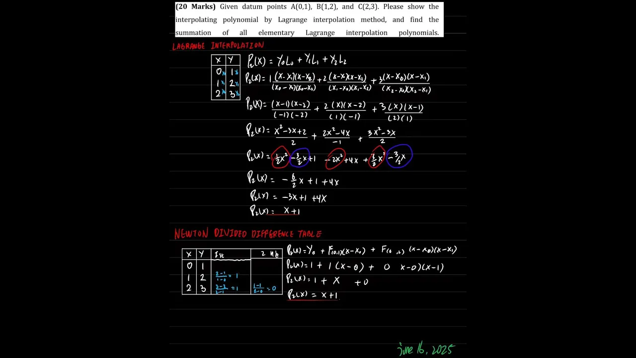
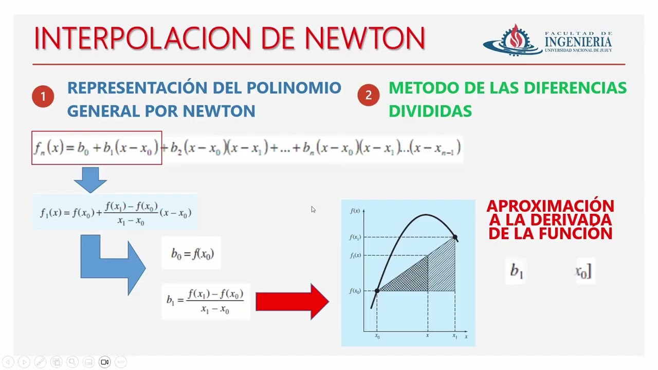
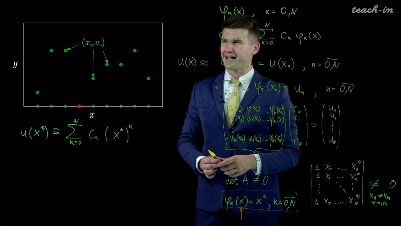
Added:Fundamentals of polynomial interpolation, such as Lagrange and Newton interpolation methods.
Runge's phenomenon and the inherent instability and oscillation issues of high-degree polynomial interpolation.
Basic calculus concepts, specifically function continuity and the physical meaning of first and second derivatives.
Linear algebra basics, including representing and solving systems of linear equations in matrix form.
Boundary conditions for cubic splines, including Clamped, Natural, and Not-a-knot boundary formulations.
Efficient numerical algorithms to solve the resulting tridiagonal system of equations, such as the Thomas Algorithm.
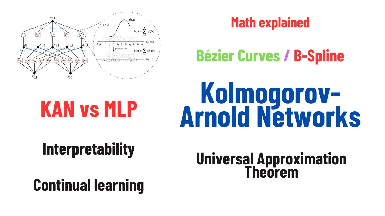
Generalizations of splines, including B-Splines and Non-Uniform Rational B-Splines (NURBS) used in CAD and computer graphics.
Multidimensional interpolation techniques, such as Bilinear and Bicubic interpolation for image processing and surface fitting.
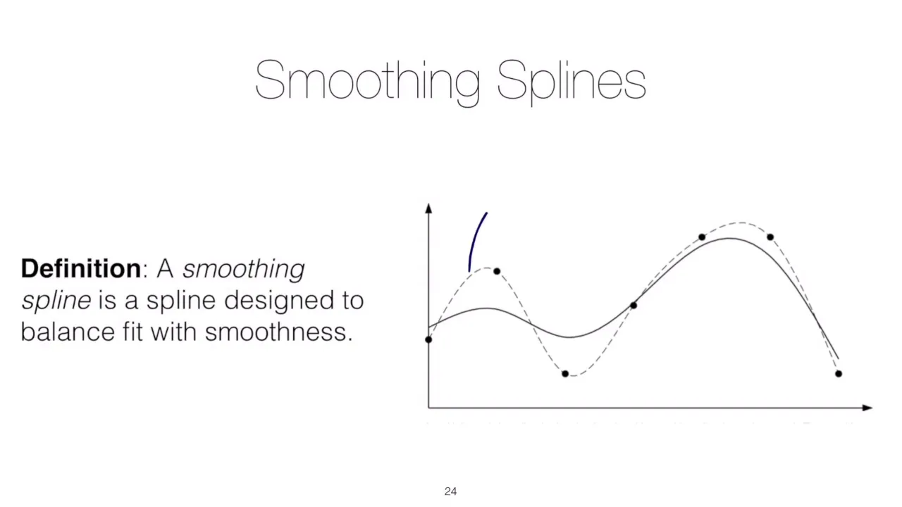
Smoothing splines and spline regression, which are used to fit curves to noisy data rather than interpolating exactly.
88.6K views1Klikes22:15Original Release: 2017-10-30
so in this video we're gonna look at spline and pearly interpolation here let's look at what is the motive you hate motivation behind moving on to another form of interpolation just done Lagrange we've done divided differences before that we looked at the vandermonde matrix so what is the motivation now it seemed from divided differences or Alec managed that just a higher order polynomial could be the way out we could efficiently perhaps using divided differences or any other like look around get higher and higher order polynomials and they would probably do the job for us it doesn't work that way as you know polynomials the higher the order of the polynomial the more you will find oscillations in the polynomial meaning meaning that it's got turning points so yeah for instance one two three four five six this could possibly possibly be a sixth order seventh order sorry one two three four five six six turning point means it could be a act some power seven that polynomial approximately not necessarily now as we go and hire a higher the order of the polynomial the more oscillations we also expect to find with that polynomial now I've got an example here and to demonstrate and this is simplest the rational function one over one plus x squared and which is drawn here for you as you can see now what I'm gonna do is I'm gonna show you how if we fit a fifteenth order polynomial to this product fifteen or sixteen order polynomial I'm not absolutely sure but somewhere around that number may be 14th through 16th order polynomial what results so have a look at this as you can see here this these are the oscillations I'm talking about if you can see here scales changed a bit but of course it's changed because of this huge jump and then coming down and then okay the approximation here pretty reasonable but look at the edges as you see at the end sorry so the ends you see huge oscillations in this polynomial and then it settles and seems to map reasonably well this is the underlying problem when we use higher order polynomials here we are using a approximately order order somewhere between 14 to 16 order 16th order polynomial so that means we're looking at something like X to the 14 or somewhere plus plus plus and so on now that's what this looks like as you can see that is not a very good approximation so it's not a great idea to necessarily used higher order polynomials because they contain oscillations this is the motivation behind why we need to look at something a little different this is where spline interpolation comes in the concept of spline interpolation is something like this you basically are take any data points that you have for instance and what you want to actually do is rather than use all the data points okay using all these data points rather than fit one polynomial to everything what you draw what you do is you limit yourself to going a point two points at a time and then between these two between these two points any two points you fit in whatever you wish for instance easiest thing would be to use a linear interpolant so a straight line basically joining these two points here's another one for these two points and then for these two and then these two and then these two so it's kind of like connect the dots which you would have played or with enjoyed possibly as a young person and this is like that I mean spline interpolation is very much like connecting the dots the only thing that you see here is this jaggedness rather abrupt turns and for instance of course I mean these types of corner these look reasonable but did this for instance looks horrible this is not what you expect in fact what you expect is more more like or like this you know you expect it to be more like you know something of a curve perhaps but one can overcome that for instance who said we have to be we have to limit ourselves to using straight lines one could very easily use some polynomial a second-order polynomial and then you know approximate all of these by second order polynomials okay and or we could go with a third order polynomial in fact and in that case um for instance choose another color here we could use a third order polynomial to approximate or between these now this is where we get the idea of linear when we use straight lines there they're called linear splines in fact these are the splines each one of these fits each one of these fits between any two points is called a spline and a linear spline is where we use a straight line between the two points and then you can have a quadratic among the nonlinear you have lots of options but again the idea is remember not to use very high order polynomials so quadratic splines would be one possible way but the most popular and most used spline seems to be the cubic spline and we would live in limit our understanding and and and in this video and the we will look at the introduction of cubic splines and how one actually tries to compute these practically so linear splines quadratic splines or cubic splines so we'll look at some of these ideas now now that situation again so what we want to do is if we want to connect these two points these two dots or these two data points with let's just change the color here so if we want to connect these two data points with a certain polynomial first of all let's start with some notation so we're going to use the letter s to denote the polynomial that fits between the data points so let's call this for instance s 0 and this one s 1 and here s 2 so you've got one two three four data points and among these you'll end up with three in fact polynomials to fit this data now there are a couple of things very simple things that you we need to keep in mind number one is s 0 and s 1 of course they're these are functions of X clearly because they're they'll end up being polynomials now one property that's very important is what happens at the juncture at this Junction here so clearly if let's say this is the point X 0 and this is the point X 1 then we clearly expect that s 0 at X 1 should be equal to s 1 and X 1 obviously because both of these are going to use the same this X 1 point it's a terminal point for the s 0 but it's a starting point for s the S 1 polynomial and s 2 doesn't contain it at all but anyway this s 0 and s 1 both being equal at this at this common point these are this is called a matching condition ok matching condition now when we want actually smoothness at these junctures at these junctions these connecting points if we want these to be smooth then one of the other requirements we usually impose on these joints so to speak are that the first derivative so the derivative at s 0 for instance at X 1 should be equal to the first derivative at X 1 of s 1 as well and similarly and similarly in fact the other requirement that the second derivative also be equal at x1 in other words in this case I mean as just as an example there's of course the other point this point here which is x2 for instance and if this was X 3 then clearly there also would be matching conditions as x2 for s1 and s2 but I'm just trying to get you to understand what the motivation the where the mathematics actually comes from is that we want smoothness at these joints now in mathematics smoothness is a is a technical term it's not just the wording in the English word but actually has some requirements and those requirements are that the first derivative exists and in fact here in this case by equating the two first derivatives we get a smooth turning point and we're requiring the second derivatives also enables the same thing which is basically to have smooth turning points here or smoothness of the joints essentially so these in fact turn out to be quite useful as you will see in a moment so let's let's look at basically so this is taken from again burden farce burden book on numerical analysis and so here I have some formal definitions and conditions that we will now look at in a much more formal manner so given a function f defined on a be some interval and a set of nodes so these are called the nodes these are all these are all nodes a is equal to x0 x1 xn to be asked Ubik spline interpolant s4 f is a function that satisfies the following condition so s FX is a cubic polynomial first of all now of course if you're using linear interpolant then s of X is a linear polynomial if you're using quadratic it could be a quadratic polynomial and so on so we are looking at cubic polynomials or cubic splines but one can apply the same ideas to in fact quadratic splines for instance denoted s G of X on the sub interval xjxj plus one so for instance X 0 to X 1 X 1 to X 2 and X 2 to X 3 so these would this this this indicates that region that range sorry of values so now we have the first this this condition is a very basic one which is a requirement that of course if the polynomial satisfies the point then SJ at any any X J which is within its range should equal F of XJ okay so that means that the data point the pair should in fact be satisfied by the polynomial within the range that you are looking at so for instance it would mean that in this example that I here that I have here that s 0 that s of X X 0 should satisfy s of X so for instance here now what I'm missing is if I say this was for the sake of argument y 0 and this was y1 for the sake of argument then what we're saying is this condition says that s 0 of X 0 should equal y 0 of course so that's what this indicates this condition basically that all the data points that you put in so and that's two at a time of course so it will be y 0 and y 1 so in both cases the polynomial that you had have should satisfy the data point that's the first one the next one then says and of course in the second here that'll be 2 so the other one would be the s 0 of x 1 equal Y 1 for instance now the next condition that you see here see is this is one of the matching conditions in fact so you see SJ plus 1 of XJ plus 1 equals s J XJ plus 1 so it's exactly this condition that I have here as that s 0 so that means if our first polynomial is s 0 ok so that should be equal to the SJ so if J was 0 then s 1 so you see s0 and s1 at the same point X 1 you see that so here you see this the two points ok XJ plus one would be the point so it's not the first point obviously it's the second point this point there is nothing before so the first time this would happen is at the second point and then at the third point it'll happen in the middle point sound okay you could have more of these but in any case that's why you see the J plus one point as the first one here it's never going to be as J or bxj on the easily okay so that's a one of the matching conditions this is a second matching condition that I showed you here and this third matching condition is this one here as in this example now this is something we didn't talk about and it's quite important and basically these are boundary conditions that are usually required and and you'll see what I'm talking about once we look at an example in fact it'll become clearer because in a cubic polynomial you're talking about four coefficients that need to be found all these conditions the data points the matching conditions provide us with conditions and their fur give us a set of simultaneous equations to find the four unknowns that we have actually it's not sorry four unknowns in fact it's you're talking about a cubic polynomial for instance just for these four data points you would have one two three polynomials cubic polynomials each one having four unknown coefficients so we'll go over the boundary conditions so here this is a special requirement there are two types of boundary conditions both of these are usually not used we use one of these boundary conditions so the first one that you see here this the second derivative at the starting point is equal to the second derivative at the endpoint now you'll notice that there is no subscript here for indicating which polynomial it is in the example I have here it would mean that the second derivative for the y 0 occurs for the s 0 polynomial range and the end point X 3 in this case appears for s 2 it doesn't appear in s 1 or s 0 remember so one has to look at where the end point actually occurs so for instance in our example this example that we have here the condition the boundary condition would be translated as second derivative at x0 which is our starting point okay it should be equal to the should be equal to zero and the third and the anti sorry the end point which is the in our case it would be s2 second derivative at X 3 in fact which is the other end point and that should be equal to zero so the this is how we would use this boundary condition so there are boundary conditions meaning at the endpoint endpoints so X 0 and X 3 being the endpoints in our this mini example that we have here now so that's one of the conditions the other condition so this is called a natural or free boundary condition and the splines that we that occur after using this type of boundary condition are called natural splines so they're called natural natural splines okay when this boundary condition is used now if we use the other ones the clamp boundary conditions now the clamp boundary conditions indicate that you know if you're provided data then you have to have the extra data of the derivative at the endpoints so for instance you need to know for instance here you need to know at s dash at x0 F dash at x0 so here in our example again it would mean that you have s 0 dash of X 0 should be equal to F dash of X 0 and the other point would be of course the other endpoint which would be in our example it would be s 2 dash of X 3 okay the endpoint should be equal to the derivative at X 3 now this is easier these this condition is easily more easily applied if we are trying to approximate a function using cubic cubic splines however if you are you it doesn't mean it's not limited to just functions one can easily fit data as well using cubic splines but in that case this tells us that if you wish to use the clamped condition you need to have the derivative the value of the derivative at the two endpoint in addition to the data that you have okay so that's something that you should note so these are the basics of cubic spline interpolation let me show you one other important important fact and and that is basically how we in fact what we in fact are looking at what is the structure of these s's okay so basically what we want to do is want to say that any SJ of X is basically equal to AJ plus BJ into X minus XJ plus CJ into X minus XJ squared the quadratic term plus a DJ into X minus XJ the cubic term so that is the structure of these SJ so for instance as an example s 0 of X would be a 0 plus B 0 into X minus X 0 plus C 0 into X minus X 0 squared plus D 0 into X minus X 0 cubed ok now let me explain let me try to give you an idea about what's going on here so this is your s 0 now in a similar way you'll get an S 1 and your s 1 is going to be looks like this now these are just two polynomials now there's a third one in our example that we have with just four data points now here you need to note something this these coefficients are unknowns there are all different unknowns so this means the third the S 2 equation will give us another 4 so we're talking about 12 unknowns here 12 unknowns and all you have are 4 data points if you insert these data points and of course you can insert these data points only in the range of values so means that only two of these points at a time so these two points for instance these two points can be inserted into s 0 so that will give you possibly two conditions to equate and so these two points then be inserted for s1 and that'll give you another two equations and and again these two points can be inserted into s2 and that'll give you another two equations so that'll give you in fact if we can't if we just look at it that that gives us six six equations possibly right and then those six equations that's not enough because we've got 12 unknowns then we would move on to our matching conditions now sometimes the matching conditions happen to overlap for instance this matching condition here overlaps with this point in fact so it doesn't really provide us with much more information however this one provides us with yet another condition another equation and this one will provide us we hope with another condition so that's two more which makes it eight now along the way usually the way these things are structured the the equations sometimes would pop out some of these constants immediately right so you would have to you would have to look at some examples to in fact look at that in a concrete manner but for instance when we look at the point x0 when you substitute in X 0 into S 0 what will happen is that all of these for instance or when you substitute X 0 years so s 0 of X 0 will be a 0 plus nothing else so that will immediately give you the 0 in fact so one of the constants is found so we are left with eleven unknowns similarly in a 1 in s 1 when we put in s 1 of X 1 that will give us in fact the value of a 1 so in this manner we can find some other contents of constants but as you can see that what is the problem at the end of the day is we need a certain number of equations to find the missing the the unknowns in fact that's why this this this boundary conditions in fact then become quite important and these matching conditions become quite important in fact as well so in the next video we'll look at a full example
Up Next
14:47
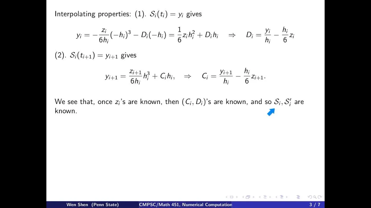
Natural Cubic Splines: Algorithm Derivation
@wenshenpsu
23.1K views•2015-02-08

4:43
Elliptic Curve Cryptography Explained: ECC, ECDSA, ECDH
@PracticalNetworking
28.5K views•2024-10-21
18:07
Cubic Spline Interpolation: Natural & Clamped Boundary Conditions
@the-Math-guy
258.1K views•2017-10-30

6:00
The Mathematical Impossibility of Accurate World Maps
@Vox
23.3M views•2016-12-02
Related Study Plans & Knowledge Roadmaps
Structured learning paths in Mathematics
mathematics
Tensor Calculus: Vectors to Riemann Curvature
01Mathematical Foundations: Linear Algebra & Calculus
02Covectors, Dual Spaces, and Tensor Basics
03The Metric Tensor and Index Gymnastics
+ 2 more learning modules
40h5 modules
Explore Roadmap
mathematics
Gödel's Incompleteness: Logic, Proofs & Limits
01Introduction to Formal Systems & Hilbert's Dream
02Set Theory, Cardinality, and Cantor's Diagonal Argument
03Arithmetization and Gödel Numbering
+ 2 more learning modules
14h5 modules
Explore Roadmap
mathematics
Galois Theory: Fields, Groups & Solvability
01Foundations of Abstract Algebra: Groups & Fields
02Polynomials & Field Extensions
03Splitting Fields & Symmetries
+ 2 more learning modules
24h5 modules
Explore Roadmap
mathematics
Non-Euclidean Geometry: Models & Geodesics
01Euclid's Fifth Postulate and the Birth of New Geometries
02Hyperbolic Space and the Poincaré Disk Model
03Geodesics: Defining Straight Lines in Curved Spaces
+ 2 more learning modules
15h5 modules
Explore Roadmap