
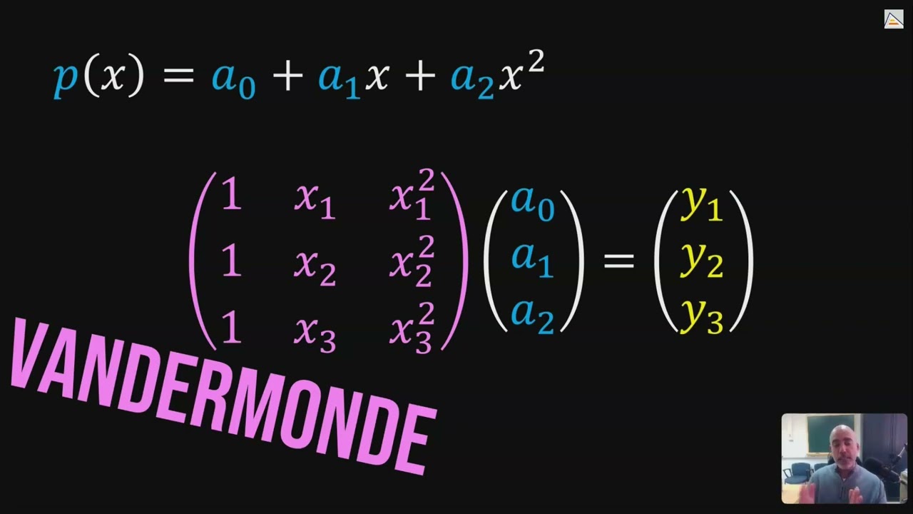









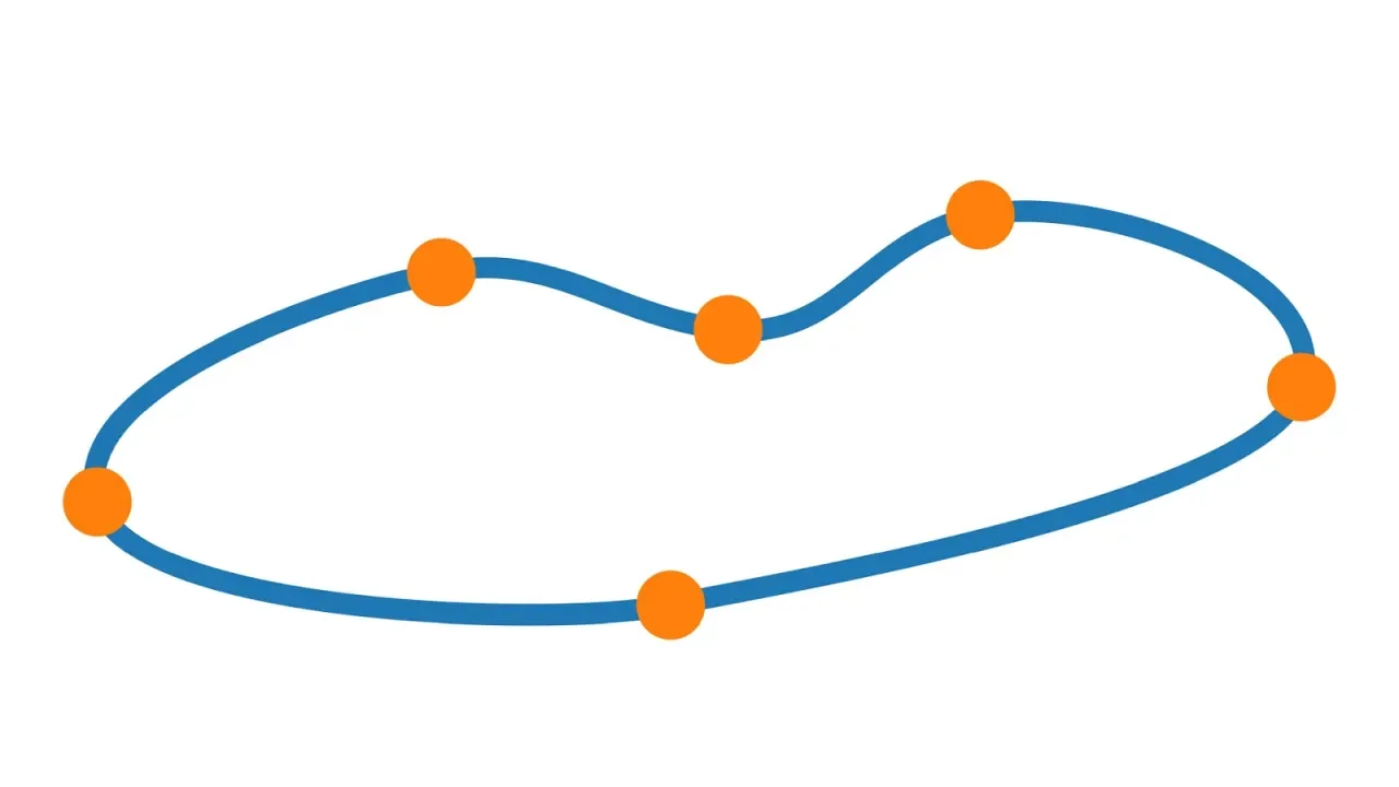





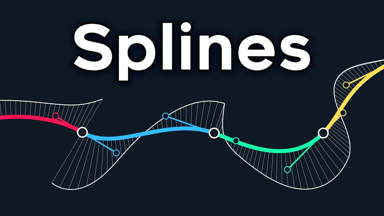


Natural cubic splines are piecewise cubic polynomials that interpolate data points with continuous first and second derivatives, where the second derivatives at the endpoints are zero; the algorithm involves defining unknown second derivative values Z_i at interior knots, expressing the spline in Lagrange form, integrating twice to obtain the cubic polynomial, applying interpolation conditions to derive relationships between coefficients, enforcing continuity of the first derivative to form a tridiagonal linear system, and solving this symmetric diagonally dominant system to find the Z_i values, which then allow computation of the complete spline.
Natural Cubic Splines: Algorithm Derivation
Added:Fundamentals of polynomial interpolation and the concept of fitting curves through a set of control points (knots).
Calculus principles of piecewise functions, continuity, and differentiability (specifically C0, C1, and C2 continuity).
Linear algebra concepts, including representing systems of linear equations in matrix form (Ax = b).
Understanding of tridiagonal matrices and the concept of linear system solvers.
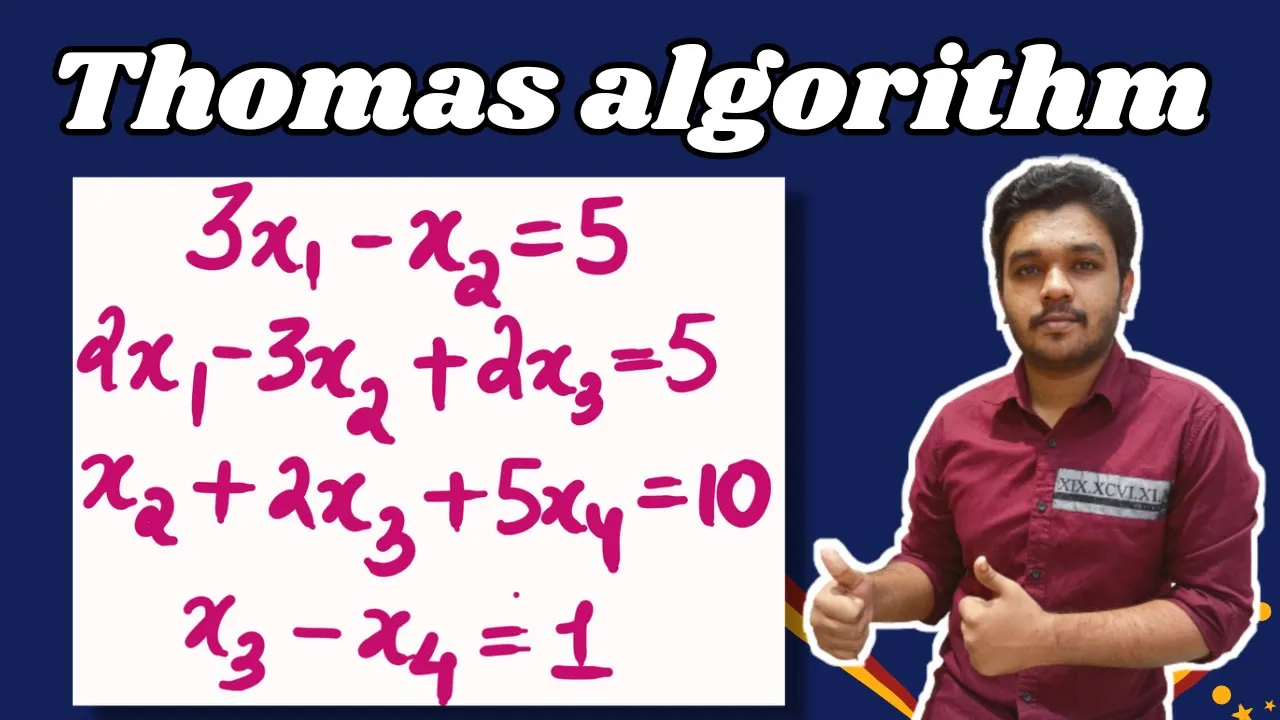
Practical implementation of the Thomas Algorithm (Tridiagonal Matrix Algorithm) to computationally solve the spline system.
Exploration of alternative boundary conditions, such as clamped, periodic, or 'not-a-knot' cubic splines.
Transitioning to B-splines (Basis splines) and NURBS (Non-Uniform Rational B-Splines) for advanced 3D modeling and computer graphics.
Application of splines to data smoothing, trajectory planning in robotics, and finite element analysis.
23.1K views170likes14:47Original Release: 2015-02-08
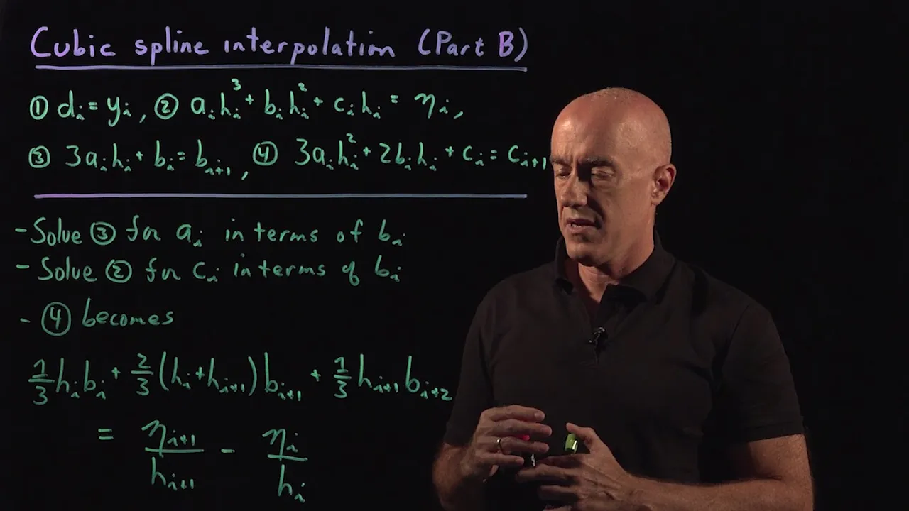
numerical computation chapter 3 video 5 in this video we will go through the derivation for the algorithm used to compute natural cubic splines so this might be a pretty long video as we out light in the previous video the algorithm is derived backwards so we start from s double derivative so let's define these values Zi Zi will be s double prime at ti4 I from 1 2 3 4 all the way to and minus 1 because Z 0 and Zn will be 0 because our condition for the natural cubic spline now we need to pay attention here these Z eyes are actually our unknowns they will be in the end our primary unknowns ok so let's use this notation H I which denote the length of the interval number I so it's TI plus 1 minus TI with that notation in hand we can write out the Lagrange form for the s double prime of I on the eyes interval so it's just a linear polynomial it's a straight line going through the Zi 2 Zi plus 1 from TI to TI plus 1 so write out its Lagrange form it takes this form so this is the Cardinal function at TI plus 1 so it's X minus T I over H I and at TI the Cardinal function is X minus TI minus 1 over negative H I where we love the negative in the front so the advantages of writing this in the Lagrange form versus the point-slope form will be clear later on in the derivation and now we're going to integrate this function once to get s Prime and then one more time to get s so we see when we reached s we did twice integrate and there shall be two arbitrary constant these two constants are really arbitrary also in the way you represent them so we have a freedom of choosing which way to represent these two arbitrary constant and here is our choice and this is actually another little trick along the way so s double prime is now written in this form and there are there is an arbitrary constant and then we write it as CI - di they are both constants and both at the time being arbitrary so um one can easily verify that taking this expression on the right hand side and differentiate it once in X and you will exactly recover the s double prime so this s prime is an antiderivative of the s double prime here and then integrate it one more time we recover the expression for si which takes this form okay so um here if you differentiate this term you got that one and if you differentiate this turn you got this one and if you differentiate this term you get CI and if you differentiate the last term you get negative di so this si is an antiderivative for this s prime so I advise you to maybe see there I'm with a piece of paper and write these functions out and check by yourself that these are actually the correct form we now check various properties that has to be satisfied by the cubic spline the first property is the interpolating property so si at T I must interpolate the value Y I so imposing that we get in the expression of si we said x equals to TI and this show you go to Y I and then the function exactly takes this form as we have here and you see the H I and each I cube can be simplified into exactly this form so we see there is no CI involved we only have a DI here and the weii is are given so one can write the DI in terms of the others so some algebraic manipulation now give me this expression for the I and next the other interpolation property on the interval from TI to TI plus one on the right at here I plus one my head I must interplay the value Y I plus one so putting in x equals to TI plus 1 in the expression of si of X I get this expression but it's just some very simple algebraic calculation and we see that di is not present and CI is the only one here and I can write CI in terms of the others some simple manipulation now gives me this form so at any point of this video you can push the pause button and to think about these algebraic manipulations and probably work it out on your own now we can conclude that once the Z eyes are numb by some way if we found the Z eyes then we can use the Z eyes to find my CIS and my D eyes and once the CIS and the eyes are none and then I can plug back in and I can find the expression for Si and s prime of I so here are actually the expressions so the SI and the s prime i after i plug in the values for CI that's a CI and that's di and then over here is CI minus di so what I did was when CI is - in the I I collect the terms containing wise together here and the turns containing Z's together here so think about it we what conditions we have not used yet we have used the property that as I interpolates the data so as is a continuous function we have used the property that as double prime interpolates the data zi so as double prime is a continuous function what about the continuity of s Prime let's check that so a spry needs to be a continuous function so it says at any inner point TI approaching from the left must equal to the value approaching from the right to TI and let's first check the value approaching from the right plugging in x equals 2 TI in the expression of si prime of X I get this expression and I see that the term here which are underlined it is actually the data so it depends on Y eyes and H eyes which will be given once your data set TI y i is given so we'll call this term here bi to shorten the notation okay so after some simplification getting rid of one of the h eyes and this simply takes this form on for s prime i at TI and now we can also write out the function as i minus 1 prime at x and then substitute X with TI and this is the that will have you might want to sit down with a piece of paper and go through the algebra to get this expression now we can set them to be equal to each other that is this expression here equals to this expression and we arrange the terms and we collect like terms because there are several Zi and we can collect them so after cleaning up and this is the expression we have so for each I from 1 2 all the way to n minus 1 the inner knots I have an equation and this equation involves 3 of such C's it evolves Zi and then it evolves the Zi minus 1 the knot on the left and the CI plus 1 on the knot on the right and we have the boundary condition Z 0 is 0 and the N is 0 so in the end this is a system of n minus 1 linear equations where my unknowns are these Z eyes see that so be careful these Z eyes are my unknowns and these H eyes are actually the coefficient so if you want to solve this in MATLAB we need to write it in matrix vector form okay so here we repeat the equations up here and then we try to write it into a matrix vector form where we call the matrix capital H and the unknown vector is Z and the right-hand side is B so let's see what is the coefficient matrix X you can see for the first row when I equals to 1 this equation will contain Z 0 Z 1 and Z 2 and since Z 0 is 0 so the first term is gone and I actually only have Z 1 and Z 2 so I have two coefficients this for the Z 1 and that's for the C 2 and then for the second row where I equals to two then I see I have actually C 1 and Z 2 and Z 3 so the coefficients in front them will be filling the position on the first column the second column and third column let's go one more step when I equals 2/3 I see that I have Z 2 Z 3 and Z 4 so the coefficients will fill in the second and the third and the fourth column which gives me H to 2 times H 2 plus H 3 and H 3 here and one can see that as I increases these triple kind of a triplet of coefficients will just move down along kind of around the diagonal so let's say you move to the second last one where you still have three these say I equals 2 n minus 2 then you will have Z n minus 3 Z n minus 2 and Z n minus 1 so which will give you this H here and 2 times these 2 H here and this age here and then for the last equation when R equals to n minus 1 we see this will be Z n which can be eliminated by using the boundary condition Z n is 0 so I have two terms Z n minus 1 and a Z and minus 2 which contributes to these two coefficients in my H matrix and outside these three diagonal line everything over here and over here there are zeros so such a matrix which has only nonzero element along the diagonal the upper diagonal and the lower diagonal it's called a tri diagonal matrix and we also notice that this is a symmetric matrix so symmetric matrix have very nice properties for example all the eigenvalues are real and we also see that this is diagonal dominant in the sense that the diagonal element in absolute value is bigger than the sum of all the off-diagonal elements adding up in absolute value which we can easily verify right so diagonal dominant matrix are non singular which means invertible which means there'll be a unique solution okay so here the Z vector will be my unknown z1 z2 z3 all the way to Zn minus 1 and the B vector is the right-hand side which is just this number here and we're filling in the corresponding place let's summarize the algorithm so in the end how would you compute it in what order so we see that we actually needed to set up the matrix vector equation first once we set it up and we have to solve it for the Z and find all the Z's and once the Z's are found and then we know we can use disease to compute the CIS and the i's and in terms we can decide what the SIS will be now programming for the code of this natural cubic spline will take quite some work so the MATLAB code for this will actually be provided to you so your job will be understanding the algorithm and then go and read the code and understand what the MATLAB code is doing and learn how to use those predefined functions that are provide to you and you may also want to take a look at the video on the mat lab simulations for the natural cubic spline ok bye see you next time
Up Next
18:07
Cubic Spline Interpolation: Natural & Clamped Boundary Conditions
@the-Math-guy
258.1K views•2017-10-30

4:43
Elliptic Curve Cryptography Explained: ECC, ECDSA, ECDH
@PracticalNetworking
28.5K views•2024-10-21

10:44
Fourier Series Introduction: The Big Idea Explained
@DrTrefor
387K views•2021-05-03

6:00
The Mathematical Impossibility of Accurate World Maps
@Vox
23.3M views•2016-12-02
Related Study Plans & Knowledge Roadmaps
Structured learning paths in Mathematics
mathematics
Tensor Calculus: Vectors to Riemann Curvature
01Mathematical Foundations: Linear Algebra & Calculus
02Covectors, Dual Spaces, and Tensor Basics
03The Metric Tensor and Index Gymnastics
+ 2 more learning modules
40h5 modules
Explore Roadmap
mathematics
Gödel's Incompleteness: Logic, Proofs & Limits
01Introduction to Formal Systems & Hilbert's Dream
02Set Theory, Cardinality, and Cantor's Diagonal Argument
03Arithmetization and Gödel Numbering
+ 2 more learning modules
14h5 modules
Explore Roadmap
mathematics
Galois Theory: Fields, Groups & Solvability
01Foundations of Abstract Algebra: Groups & Fields
02Polynomials & Field Extensions
03Splitting Fields & Symmetries
+ 2 more learning modules
24h5 modules
Explore Roadmap
mathematics
Non-Euclidean Geometry: Models & Geodesics
01Euclid's Fifth Postulate and the Birth of New Geometries
02Hyperbolic Space and the Poincaré Disk Model
03Geodesics: Defining Straight Lines in Curved Spaces
+ 2 more learning modules
15h5 modules
Explore Roadmap