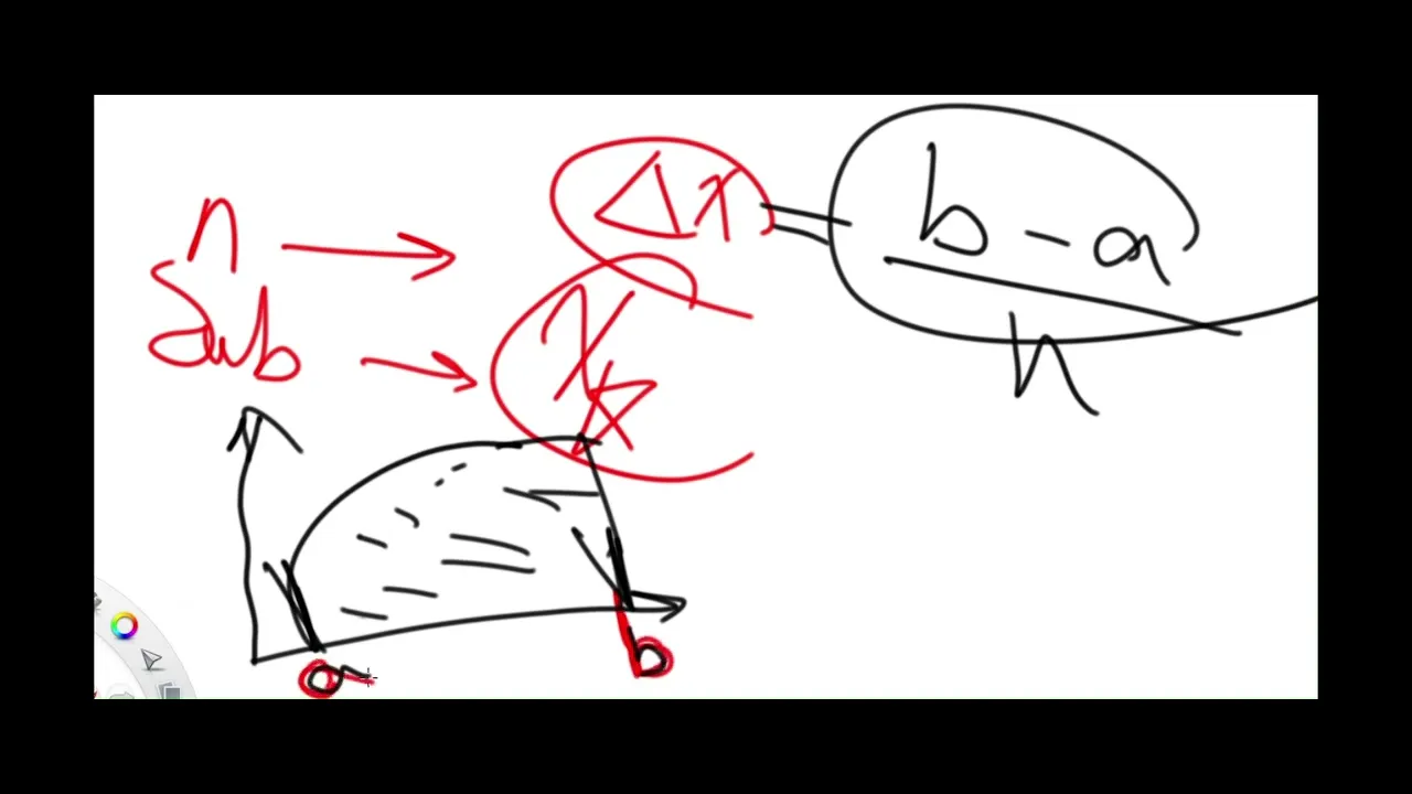
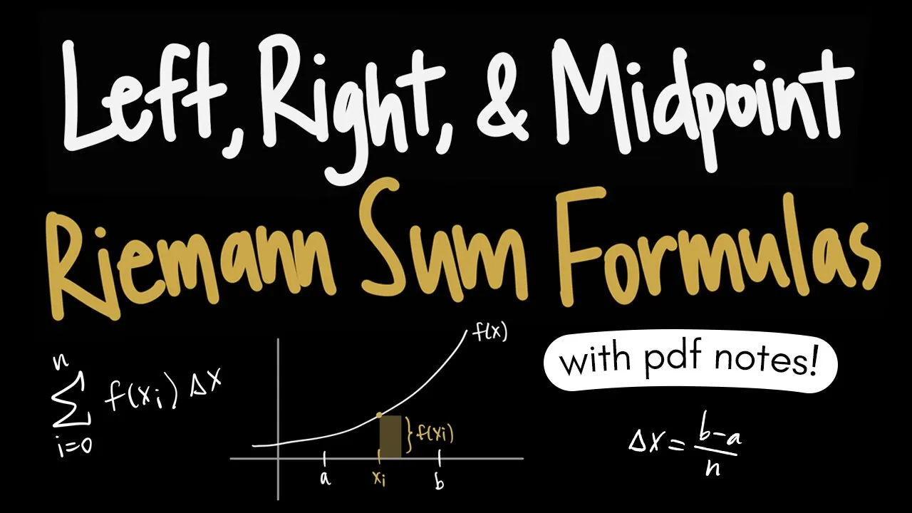
Simpson's Rule & Numerical Integration | Calculus Tutorial

This section covers advanced numerical integration techniques. Romberg Integration is a recursive method that improves upon the Trapezoidal Rule using Richardson extrapolation. The process involves applying Trapezoidal Rule with h, h/2, h/4, etc., then using formulas: R(h) = (4T(h/2) - T(h))/3 for the second column, and R(h) = (16R(h/2) - R(h))/15 for the third column. The stopping condition is when two successive values become equal. The instructor demonstrates this with ∫₀¹ (1+x²) dx, showing how the table converges to the exact value 4/3 ≈ 1.3333. Gaussian Quadrature approximates integrals using weighted sums at specific Gauss points. For [-1, 1]: x₀=-1, w₀=1; x₁=0, w₁=2; x₂=1, w₂=1. For x=√3/5: ∫f(x)dx ≈ (5/9)f(-√3/5) + (8/9)f(0) + (5/9)f(√3/5). For non-standard intervals, use transformation: x = (b-a)t/2 + (b+a)/2, dx = (b-a)/2 dt. The instructor demonstrates with ∫₀¹ (4x² + x) dx.

This comprehensive lesson covers two advanced numerical integration methods. Romberg integration improves the trapezoidal rule by adding correction factors, with the formula using 4^k for the next level minus the previous level, divided by 63. The trapezoidal rule calculates integrals by summing endpoints and twice interior points, multiplied by height. MATLAB implementation involves creating x values using linspace, evaluating the function, and applying the Romberg correction: T_new = (4^k × T_current - T_previous) / (4^k - 1). Gauss quadrature minimizes integration error by making upper and lower bounds movable, using pre-computed tables with coefficients and roots for the interval [-1, 1]. When the integral is not from -1 to 1 but from a to b, a change of variable is required: x = (b-a)/2 × t + (b+a)/2, and dx = (b-a)/2. The integral becomes: (b-a)/2 × ∫_{-1}^1 f((b-a)/2 × t + (b+a)/2) dt.

This segment covers advanced numerical integration techniques including Romberg integration, which improves the accuracy of the trapezoidal rule by using Richardson extrapolation. The instructor explains how this method combines results from different partition sizes to eliminate error terms systematically. The video also introduces Gaussian quadrature, a numerical integration method that approximates integrals by evaluating the function at specific optimally chosen points (nodes) and weighting these values. Unlike methods using equally spaced points, Gaussian quadrature uses optimally chosen points that minimize error for a given number of function evaluations, making it particularly efficient for smooth functions.

Romberg integration is a numerical technique that systematically improves the accuracy of integral approximations by applying Richardson extrapolation to the composite trapezoidal rule, generating a triangular table where each entry R(k,j) = R(k,j-1) + [R(k,j-1) - R(k-1,j-1)]/(4^(j-1)-1), with the final entry in the bottom-right corner providing the most accurate approximation of order h^(2n).

This comprehensive lesson covers two powerful numerical integration techniques. Richardson extrapolation systematically improves integral accuracy by combining results from different step sizes, with each correction increasing error order by two (h² → h⁴ → h⁶ → h⁸). The error ratio follows predictable patterns (2, 16, 64 for doubling segments), enabling derivation of correction formulas with coefficients 2ᵏ/(2ᵏ-1) and -1/(2ᵏ-1). After the second correction, results achieve approximately seven digits of accuracy. Gaussian quadrature addresses the trapezoidal rule's endpoint limitation by selecting optimal evaluation points within the interval. For the two-point Gauss-Legendre method, solving a system requiring exact integration of constant, linear, quadratic, and cubic functions yields x₀ = -1/√3 and x₁ = 1/√3, with coefficients c₀ = c₁ = 1. This achieves third-order accuracy (exact for polynomials up to degree 3) using only two function evaluations, representing a fundamental improvement over endpoint-based methods.

The Simpson's rule can be implemented in MATLAB with a function that takes inputs: the function handle, x0, xn, and step size h. The function generates x values, computes y values at each point, then applies the Simpson's formula. The instructor shows how to calculate the error estimate using the formula: Error = (h^4/180) * max|f''''(x)|, where f'''' is the fourth derivative. The code demonstrates handling the alternating coefficients (4 for odd indices, 2 for even indices) and computing the final integral value.

Apply Simpson's Rule by calculating Δx = (b-a)/n = 0.5 for [0,5] with n=10. Generate x-values: 0, 0.5, 1.0, 1.5, 2.0, 2.5, 3.0, 3.5, 4.0, 4.5, 5.0. Apply the Simpson's formula: S₁₀ = (Δx/3)[f(x₀) + 4f(x₁) + 2f(x₂) + 4f(x₃) + 2f(x₄) + 4f(x₅) + 2f(x₆) + 4f(x₇) + 2f(x₈) + 4f(x₉) + f(x₁₀)]. Remember the coefficient pattern: endpoints get 1×, odd indices get 4×, even indices get 2×.

Simpson's Rule approximates definite integrals by fitting parabolic curves (polynomials of degree 2) to consecutive sets of three points, rather than using straight lines like the trapezoidal rule. The method requires an even number of subintervals (2n) and an odd number of points (2n+1), with the formula: ∫f(x)dx ≈ (h/3)[f(x₀) + 4f(x₁) + 2f(x₂) + 4f(x₃) + ... + 4f(x₂n-1) + f(x₂n)], where h is the subinterval width. This approach provides better accuracy than single polynomial interpolation because it avoids the Runge phenomenon by using local parabolic approximations. The Python implementation demonstrates how to construct the partition, apply the weighted sum formula, and achieve high precision (14+ decimal places) with sufficient subintervals.

Simpson's method is a numerical integration technique used when analytical integration is not possible. The method approximates the definite integral by replacing the curve between three consecutive points with a second-order polynomial (parabola). The algorithm involves: (1) dividing the interval into an even number of subintervals, (2) approximating each pair of subintervals with a parabolic segment, (3) determining polynomial coefficients by solving a system of equations from three consecutive points, (4) calculating elementary areas under each parabolic segment, and (5) summing all elementary areas. The final formula provides a direct expression for the integral. In MATLAB implementation, the method requires an even number of intervals and produces exact results for polynomials of degree 3 or less, as demonstrated by integrating f(x) = 3x² + 6 over [0, 2], which yields the exact analytical result of 10.

This comprehensive segment covers the complete implementation of Simpson's 1/3 Rule in MATLAB. The instructor introduces the rule as a numerical integration technique for approximating definite integrals when analytical solutions are difficult. The function requires four inputs: f(x) (the function to integrate), A and B (integration limits), and N (number of sub-intervals, which must be even). The mathematical formula is: ∫f(x)dx = (H/3) × [y₀ + yₙ + 2(y₂ + y₄ + ... + yₙ₋₂) + 4(y₁ + y₃ + ... + yₙ₋₁)], where H = (B - A)/N. The implementation involves calculating sub-interval width H, generating x-values, computing function values using MATLAB's subs function, and implementing loops with if-else conditions to apply the correct weights (2 for even-indexed terms, 4 for odd-indexed terms). The final result is calculated as I = (H/3) × sum.

Numerical integration applies to real-world data tables where functions aren't explicitly known. For n data points, trapezoid/Simpson's use all n points while midpoint uses n/2 points. Example: Water flow rate data at times 0,5,10,15,20,25,30 minutes (7 points) requires n=6 for trapezoid/Simpson's and n=3 for midpoint. With Δx=5, T₆ = 2.5×[12.3 + 2×(12.7+13.1+13.3+13.5+13.2) + 13.1] = 392 gallons. S₆ = (5/3)[12.3 + 4×(12.7+13.3+13.2) + 2×(13.1+13.4) + 13.1] = 392 gallons. M₃ = 10×(12.7+13.3+13.2) = 392 gallons. All methods yield identical results here.

Integration has important physical applications including: (1) Work: W = ∫ from a to b of F(x)·dx, where F is force, (2) Center of mass: requires integrating position weighted by density, (3) Pressure: P = ∫ from a to b of F(x)/A(x)·dx. These applications demonstrate how integration solves real-world physics problems.

For continuous density functions, calculate the total mass using M = ∫ρ(x)dx and the center of mass using x̄ = (∫xρ(x)dx) / M. The numerator involves integrating position times density. With discrete data, use Riemann sums: sum (x_i × ρ(x_i) × Δx) for the numerator and sum (ρ(x_i) × Δx) for the denominator. The result gives the balancing point, which makes intuitive sense - higher density regions pull the center of mass toward them.

Work (usaha) is the product of force and displacement. For constant force, W = F × X. For variable force, use integration: W = ∫ from a to b of F(x) dx. For springs, W = (1/2)k(Δx)². Hydrostatic pressure is P = ρgh, and force on a surface is F = P × A. For curved surfaces, integrate pressure over area. Work to pump fluid equals work to lift fluid to exit point: W = ∫ ρg × A(y) × h(y) dy. Center of mass is the weighted average position. For discrete particles: X_cm = (Σ m_i x_i) / (Σ m_i). For continuous systems: X_cm = (∫ x dm) / (∫ dm). For 1D objects with density λ(x), dm = λ(x) dx. For 2D laminas with density σ(x,y), dm = σ(x,y) dA.

This section covers two fundamental calculus applications. First, the trapezoid rule estimates definite integrals using trapezoids: for n=4 intervals from x=0 to x=4 with Δx=1, the formula (Δx/2)[f(x₀) + 2f(x₁) + 2f(x₂) + 2f(x₃) + f(x₄)] yields an estimate of 10. Second, the center of mass for a wire with variable density ρ(x) is found by dividing the moment M = ∫xρ(x)dx by the total mass m = ∫ρ(x)dx. For ρ(x) = 6(x-1) on [1,3], the center of mass is at x̄ = 28/12 = 7/3 ≈ 2.33, demonstrating how weighted averages determine equilibrium points.