In biomechanics, to calculate unknown muscle and joint forces in a lever system like the calf raise, take moments about one of the unknown force points to eliminate it from the equation; for example, taking moments about the ankle joint cancels the joint reaction force, allowing you to solve for the calf muscle force using the equation ΣM = 0, where the muscle force creates a clockwise moment and the body weight creates a counterclockwise moment, then verify the joint reaction force using vertical force equilibrium ΣFy = 0.
Calf Muscle & Ankle Joint Reaction Forces: Foot Up Calculation
Added:Deep Dive
Fundamentals of Static Equilibrium: Understanding how to apply Newton's First Law to systems in static balance, specifically summing forces and moments to zero.

الصف الثاني الثانوي 🔥المراجعه النهائية🔥شرح الاتزان كله في فيديو واحد🔥#الاتزان #المراجعه_النهائية
89.8K
Static equilibrium requires that the net force on a body equals zero. For two forces: they must be equal in magnitude, opposite in direction, and collinear. For three forces: they must be concurrent (intersect at a single point). The resultant of any two forces must equal the third force in magnitude and opposite in direction. The Triangle of Forces method states that if a body is in equilibrium under three concurrent forces, and a triangle is drawn with sides parallel to the lines of action of the forces in a consistent direction, then the lengths of the sides are proportional to the magnitudes of the corresponding forces. Lami's Theorem states that the magnitude of each force is proportional to the sine of the angle between the other two forces: Q1/sin(α) = Q2/sin(β) = Q3/sin(γ).
Click to watch →

ESTÁTICA PROBLEMAS
17.3K
A body is in equilibrium when it has no acceleration, occurring either at rest (static equilibrium) or moving with constant velocity (dynamic equilibrium). The first condition of equilibrium requires that the sum of forces to the right equals the sum to the left, and the sum upward equals the sum downward. This principle forms the foundation for solving statics problems where bodies remain stationary or move uniformly.
Click to watch →

مراجعة الإتزان
694
Static equilibrium problems involve stationary bodies with given and unknown values. Two fundamental laws govern equilibrium: (1) Force equilibrium - sum of downward forces equals sum of upward forces; if forces are unbalanced, the body moves in the direction of the greater force. (2) Moment equilibrium - sum of clockwise moments equals sum of counterclockwise moments; if moments are unbalanced, the body rotates. To solve problems, choose a pivot point, calculate all moments at that point, and determine their directions.
Click to watch →

contrôle 1 physique tronc commun 2eme semestre
70.9K
This section covers the foundational principles of static equilibrium in physics. The key concepts include: (1) The conditions for equilibrium require forces to act in the same plane; (2) When a body has negligible mass (like a light paper), gravitational force becomes insignificant and can be neglected in calculations; (3) Forces must be properly identified and labeled for analysis; (4) The weight of a body equals mass times gravitational acceleration (W = mg); (5) For equilibrium, the sum of all forces must equal zero. These principles form the basis for analyzing any static system where bodies remain at rest.
Click to watch →
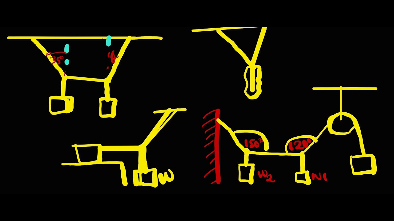
Dynamics (Staric Equilibrium Part 1)
202
Static equilibrium occurs when an object is not moving. The first condition requires that the summation of all forces equals zero (∑F = 0), meaning forces in opposite directions must balance each other. The second condition requires that the summation of all torques equals zero (∑τ = 0). To solve equilibrium problems, draw a Cartesian coordinate system and resolve all forces into their x and y components. For vertical equilibrium, upward forces equal downward forces; for horizontal equilibrium, forces in opposite horizontal directions must cancel.
Click to watch →
Deep Dive
Constructing Free Body Diagrams (FBDs): The ability to isolate a biological segment (such as the foot) and represent all acting external forces, joint reactions, and muscle tensions.

Night Marathon | Complete Engineering Mechanics - 2 | By Apuroop Sir
33.8K
A Free Body Diagram (FBD) is a graphical representation showing all forces acting on a body. To construct an FBD: (1) Identify the body of interest, (2) Draw the body as a simple shape, (3) Identify all forces acting on it (gravity, normal force, friction, applied forces, tension), (4) Draw arrows representing each force with appropriate direction and magnitude. FBDs are essential for applying Newton's laws to solve mechanics problems.
Click to watch →
EM&SM || SOM II Unit 1 || One Shot || Clear All Doubts By Gaurav Sir
2.2K
A Free Body Diagram (FBD) is a graphical representation showing all forces acting on a body. To construct an FBD: (1) Isolate the body from its surroundings, (2) Remove all contact surfaces, (3) Replace each contact with its reaction force (perpendicular to the surface), (4) Include all applied forces and the body's weight. All reaction forces should act from the point of contact.
Click to watch →

9 Forces and Laws of Motion | Introduction
427
A free body diagram (FBD) is a sketch showing all forces acting on an object using lines and arrows, without drawing the actual object. To construct an FBD: identify the object, draw arrows representing all forces acting on it (not forces the object exerts on others), and label each force with its magnitude and direction. For example, when two people push a car, draw arrows from the car representing each person's force, plus any opposing force. Arrows show direction and relative magnitude. This visual tool helps analyze forces and apply Newton's laws to solve problems.
Click to watch →
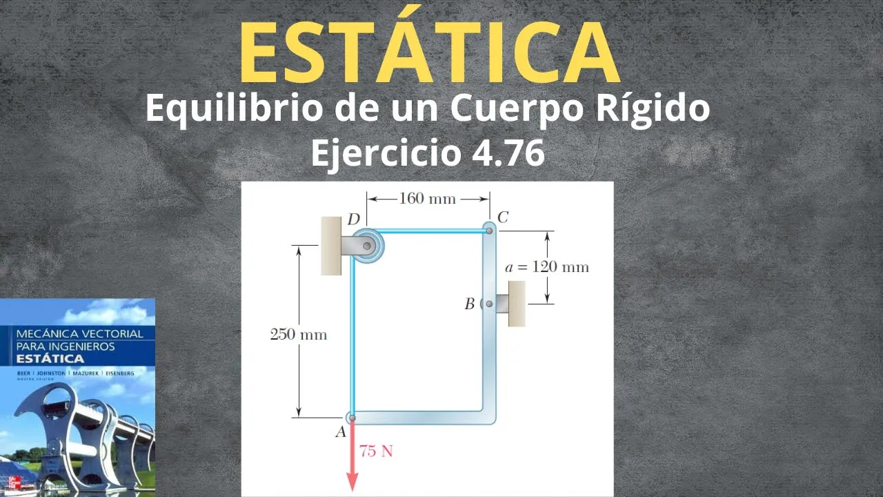
ESTÁTICA: Equilibrio de un Cuerpo Rígido | Ejercicio 4.76 Beer and Johnston 9 ed #estática
1K
A Free Body Diagram (FBD) is a graphical representation of all forces acting on a body. To construct an FBD: (1) isolate the body from its surroundings, (2) draw all external forces including applied loads and support reactions, (3) indicate the direction of each force, and (4) label all known and unknown forces. The FBD is the foundation for applying equilibrium equations.
Click to watch →

2.3 Drawing Force Body Diagrams (FBDs) + 10 Common FBDs to Know
262
A Free Body Diagram (FBD) is a visual representation of all forces acting on an object, drawn as a dot with arrows representing each force vector; to draw an FBD correctly, identify the object, represent it as a dot, draw all forces acting on it (including weight mg, normal force perpendicular to surfaces, friction opposite to motion, tension from ropes/cables, and applied forces), and ensure forces are balanced or unbalanced according to the object's motion state (zero net force means no acceleration, non-zero net force means acceleration in that direction).
Click to watch →
Deep Dive
Torque and Moment Arm Calculations: Knowing how to calculate torque using force magnitude, direction, and the perpendicular distance from the pivot center (the ankle joint).

AP- torque
372
The moment arm is the perpendicular distance from the axis to the line of action of the force. It equals R sin φ, where φ is the angle between R and F. Torque can be calculated as the product of force and moment arm: τ = F × (R sin φ). This is mathematically equivalent to τ = R × F sin φ. The moment arm concept provides an alternative way to visualize torque as the force multiplied by the effective lever arm.
Click to watch →

Rotation Part 2: Video 3 - Using the Moment Arm to Calculate Torque
489
Torque is the twist a force gives to a rotating object, describing its effectiveness in changing rotational motion. The moment arm is the perpendicular distance from the center of rotation to the line of force, found by drawing an infinite line through the force vector and dropping a perpendicular from the center of rotation. A sign convention designates counterclockwise torques as positive and clockwise as negative. The torque formula is τ = ± R⊥ × F, where R⊥ is the moment arm and F is the force magnitude. In an example, a 50N force applied horizontally to a table's top edge, with the center of rotation at the bottom of the left leg and moment arm of 0.8m, produces a clockwise torque of -40 N·m.
Click to watch →

Lecture 2 | Biomechanics (1)
5.8K
Torque (moment of force) is the rotational effect of a force, calculated as the product of force and moment arm (τ = F × d). The moment arm is the perpendicular distance from the line of action of a force to the axis of rotation. Forces can be resolved into components using trigonometric functions (sine and cosine). Understanding these calculations is essential for analyzing rotational movements and designing effective interventions.
Click to watch →

2 Aprel 2023 Kaspi kursları Blok sınaq imtahanı qrup I sinif XI Fizika suallarının izahı
861
Torque (moment) is calculated as the product of force and the perpendicular distance from the pivot point (moment arm). When forces are applied at different distances from the pivot, the torque varies proportionally with the distance. Forces whose lines of action pass through the pivot point produce zero torque.
Click to watch →

NSCA Certified Personal Trainer Exam | Chapter 4 Breakdown |
446
Torque (also called moment of force) is the rotational force that causes movement around joints. The formula is: Torque = Force × Moment Arm. The moment arm is the distance from the pivot point (joint) to where the force is applied. A longer moment arm means more torque and a harder lift. In a bicep curl, the moment arm is the horizontal distance from the elbow to the dumbbell, which changes throughout the lift and is longest when the forearm is parallel to the floor.
Click to watch →
Deep Dive
Basic Anatomy of the Lower Limb: Familiarity with the anatomical relationship between the calf muscles (gastrocnemius/soleus), the Achilles tendon, the ankle joint center, and the metatarsal heads.

Chp1 | Lower Limb Introduction | BD Chaurasia Regional Anatomy | Dr Asif Lectures
125.6K
The lower limb shares basic structural organization with the upper limb but has fundamentally different functions. While the upper limb specializes in grasping and fine motor movements, the lower limb is primarily designed for weight-bearing and locomotion. In the anatomical position, the lower limb is positioned with the foot pointing forward and the leg slightly abducted. The anterior surface faces forward, the posterior surface faces backward, the medial surface faces toward the midline, and the lateral surface faces away from the midline. The lower limb consists of four main regions: the thigh (femur), leg (tibia and fibula), ankle (tarsal bones), and foot (metatarsals and phalanges). Each region contains specific bones and joints. The thigh contains the femur, forming the hip joint proximally and knee joint distally. The leg contains the tibia and fibula, forming the knee joint proximally and ankle joint distally. The ankle contains the tarsal bones (talus, calcaneus, navicular, cuboid, and three cuneiforms), forming the ankle joint proximally and intertarsal joints distally. The foot contains the metatarsals and phalanges, forming the metatarsophalangeal and interphalangeal joints.
Click to watch →
Anatomy of Lower Limb - Quick Review - Anatomy Review Series
448.4K
The lower limb exhibits anatomical opposition to the upper limb, with hip flexion moving the thigh backward unlike shoulder flexion. The thigh contains three compartments: anterior (quadriceps and sartorius for hip flexion/knee extension, supplied by femoral nerve), medial (adductors for hip adduction, supplied by obturator nerve), and posterior (hamstrings for knee flexion, supplied by sciatic nerve). The leg has three compartments: anterior (tibialis anterior, extensors for dorsiflexion, supplied by deep fibular nerve), posterior (gastrocnemius, soleus, plantar flexors, supplied by tibial nerve), and lateral (fibular muscles for eversion, supplied by superficial fibular nerve). The lumbosacral plexus bridges lumbar and sacral nerves via the lumbosacral trunk, with dermatomes progressing from T10 (umbilicus) through L5 to S2. Vascular supply follows the external iliac → femoral → popliteal → anterior/posterior tibial arteries, while venous drainage includes the great saphenous vein. Lymphatic drainage terminates in the femoral lymph node group.
Click to watch →

Lower Limb: Surface Anatomy & Osteology – Anatomy | Lecturio
164.9K
The lower limb consists of the gluteal region (hip bone formed by ilium, ischium, and pubis), thigh (femur with head, neck, trochanters, and condyles), leg (tibia and fibula with tibial plateau, malleoli, and fibular head), and foot (tarsal bones including calcaneus, talus, navicular, cuboid, and cuneiforms, metatarsals, and phalanges), enabling movements such as hip flexion/extension, abduction/adduction, rotation; knee flexion/extension and rotation; ankle dorsiflexion/plantarflexion, inversion/eversion; and toe movements.
Click to watch →

Lower Limb Muscles || Anatomy || Live Streaming By Dr. Krishna
91.1K
The lower limb anatomy begins at the inguinal ligament, which extends from the anterior superior iliac spine to the pubic tubercle. The lower limb is divided into three main regions: the thigh (containing the femur bone), the leg (containing the tibia and fibula), and the foot. Key bony landmarks include the anterior superior iliac spine, pubic tubercle, pubic crest, and pubic symphysis. Understanding these foundational anatomical relationships is essential before studying the detailed muscle compartments of the thigh.
Click to watch →

Introduction to lower limb muscles anatomy
188.1K
The lower limb contains muscles organized by their primary actions at the hip, knee, ankle, and foot joints; hip muscles include flexors (psoas major, iliacus, rectus femoris, sartorius), extensors (gluteus maximus, hamstrings), abductors (gluteus medius, minimus), and lateral rotators (six muscles including piriformis); knee muscles consist of quadriceps femoris (extensors) and hamstrings (flexors); ankle and foot muscles include gastrocnemius and soleus for plantar flexion, tibialis anterior for dorsiflexion, and various muscles for toe movement and foot inversion/eversion.
Click to watch →
Prerequisite Knowledge
- Concept 01Fundamentals of Static Equilibrium: Understanding how to apply Newton's First Law to systems in static balance, specifically summing forces and moments to zero.
- Concept 02Constructing Free Body Diagrams (FBDs): The ability to isolate a biological segment (such as the foot) and represent all acting external forces, joint reactions, and muscle tensions.
- Concept 03Torque and Moment Arm Calculations: Knowing how to calculate torque using force magnitude, direction, and the perpendicular distance from the pivot center (the ankle joint).
- Concept 04Basic Anatomy of the Lower Limb: Familiarity with the anatomical relationship between the calf muscles (gastrocnemius/soleus), the Achilles tendon, the ankle joint center, and the metatarsal heads.
Subsequent Learning
- Step 01Dynamic Biomechanical Modeling: Transitioning from static equilibrium to dynamic analysis (inverse dynamics) to calculate joint forces during walking, running, or jumping.
- Step 02Lever Systems and Mechanical Advantage: Analyzing the foot-ankle complex as a lever system and calculating its mechanical advantage under different postural configurations.
- Step 03Tissue Mechanics (Stress and Strain): Applying calculated force values to estimate the tensile stress on the Achilles tendon and the compressive stress on the ankle's articular cartilage.
- Step 04Clinical Biomechanics and Injury Analysis: Using force calculations to assess the risk of pathologies such as Achilles tendinopathy, plantar fasciitis, and ankle osteoarthritis.
Force Analysis
Joint Reaction
Force Analysis
0:01Playing Section
- 1
Applies static equilibrium to calf exercise.
- 2
Takes moments about joint to cancel unknown.
- 3
Solves for muscle force using distances.
Limitations of Static Equilibrium and Single-Muscle Biomechanical Models
While static equilibrium models provide a foundational introduction to biomechanics, they significantly oversimplify the human musculoskeletal system. Critics point out that static calculations fail to account for dynamic variables such as acceleration, inertia, and the viscoelastic properties of tendons (like the Achilles tendon), which store and release energy. Furthermore, the ankle-foot complex is statically indeterminate; simple lever models assume the calf muscles act in isolation to resist gravity. In reality, movement involves muscle co-contraction (simultaneous activation of agonists and antagonists like the tibialis anterior) to stabilize the joint. Modern biomechanical analysis favors dynamic, multi-segment modeling and EMG-driven simulations to accurately capture true joint reaction forces and muscle synergy.
Deep Dive
Dynamic Biomechanical Modeling: Transitioning from static equilibrium to dynamic analysis (inverse dynamics) to calculate joint forces during walking, running, or jumping.

Rhino User Webinar: The Vivobarefoot BIOME project
2.5K
Capturing dynamic foot behavior requires combining static scan data with biomechanical knowledge, pressure maps, and understanding of how feet change under load—a foot can exert up to four times body weight during certain movements. The system combines hardcoded numerical values with dynamic percentages across the foot surface, representing years of iterative refinement balancing simplicity for users with accuracy for results. The system integrates with scanning partners like Volumental, accepting various scan sources while remaining agnostic to input formats. Repeated scanning enables longitudinal monitoring of foot health over time, aggregating multiple scans to create more accurate representations of individual feet. As feet change due to activity, age, or treatment, the system can adapt designs accordingly—for compromised feet, this enables progressive correction by adjusting deform class methods to gradually improve biomechanics through footwear design. The system implements customer scanning infrastructure through in-store scanners and mobile options, though mobile scanning presents resolution challenges. The foot-centric approach benefits traditional manufacturing methods beyond additive production—designers can create concepts in images that instantly propagate to all lasts, replacing the traditional months-long process of updating molds.
Click to watch →

Introducción a la Biomecánica: Dr. Samuel Sánchez Caballero . Profesor de la UPV
30.5K
Biomechanical models are mathematical representations using Newton's laws to reproduce real conditions. Simple models provide useful conclusions while complex models (representing multiple muscles) offer greater detail. Inverse kinematics matches model kinematics to captured motion by minimizing position errors between model markers and actual positions. Inverse dynamics calculates joint forces and moments from kinematic data through time differentiation, revealing loads transmitted through joints. Joint forces vary with angle, typically reaching maximum values when adjacent joint angles are minimum. This explains injury mechanisms, such as vertebral injuries in American football when players lower heads and receive frontal impact, transmitting all load through the spine since muscles are not working.
Click to watch →
biomechanics of bicep tear
19.8K
Bicep tear analysis requires both static and dynamic approaches. In a 135 lb preacher curl case, static analysis yielded 18.26 MPa stress, while dynamic analysis (accounting for 5.5 rad/s² angular acceleration) increased this to 29.2 MPa—60% greater. This demonstrates that dynamic factors significantly increase tendon stress. The value remains below the 50-150 MPa failure range, suggesting shear stress and fatigue from prior heavy attempts contributed to failure.
Click to watch →

La Biomeccanica sui Social è Quasi Tutta Sbagliata? (con Paolo Evangelista)
6.7K
Static biomechanical analysis (drawing arrows on single frames) cannot explain dynamic phenomena like the sticking point. Dynamic analysis requires considering accelerations, velocities, and time-dependent changes in forces. When accelerations are zeroed (static conditions), equations become much simpler. True biomechanics involves differential equations and complex mathematical analysis that most people cannot comprehend.
Click to watch →
Euphoria Physics Engine
192.7K
Euphoria represents a paradigm shift in game character animation by implementing biomechanical AI that gives characters central nervous systems, brains, spinal cords, and muscles. This enables reflexive, self-preservation behaviors where characters autonomously react to threats like falling by grabbing beams or other characters. Unlike traditional animation systems, Euphoria calculates interactions in real-time rather than playing pre-recorded sequences, creating unpredictable and unique responses each time. Characters possess environmental awareness where both parties influence each other—Stormtroopers know beams exist while beams respond to weight by splintering and breaking. This technology originated from Oxford University research simulating human and animal movement, evolving from simple creatures learning to walk into sophisticated autonomous agents capable of complex, realistic interactions.
Click to watch →
Deep Dive
Lever Systems and Mechanical Advantage: Analyzing the foot-ankle complex as a lever system and calculating its mechanical advantage under different postural configurations.

Basit Makineler -11. sınıf - MEB uyumlu - Soru çözümlü #aytfizik #basitmakine #fiziikkonuanlatım
60.2K
Levers consist of a rigid bar pivoting around a fulcrum. Mechanical advantage depends on fulcrum position relative to load and effort. When fulcrum is in the middle (seesaw), no force gain occurs but direction changes. When fulcrum is at one end (wheelbarrow), force gain is achieved because effort arm is longer. When fulcrum is closer to effort (scissors), force is lost but distance moved is reduced. The mechanical advantage equals the ratio of effort arm length to load arm length.
Click to watch →

BASİT MAKİNELER 0'DAN AYT FİZİK KONU ANLATIMI VE SORU ÇÖZÜMÜ| AYT FİZİK ÇEKAP KAMPI BASİT MAKİNELER
69.5K
Mechanical advantage for levers is calculated as MA = load/force = distance_force/distance_load. To increase mechanical advantage, increase the distance from the fulcrum to the applied force or decrease the distance from the fulcrum to the load. For complex systems, analyze from the load upward through each component. The total mechanical advantage is the product of individual mechanical advantages. When pulleys and levers are combined, the total mechanical advantage is the product of individual mechanical advantages. For example, a lever with MA = 2 combined with a pulley system with MA = 3 gives total MA = 6.
Click to watch →

Basit Makineler | 30, 31 ve 32. Gün | 2026 | 90 Günde AYT Fizik Kampı
45.3K
Levers are simple machines consisting of a rigid bar that pivots around a fulcrum. The mechanical advantage depends on the ratio of force arm to load arm. If force arm > load arm, force gain occurs (MA > 1). If force arm < load arm, distance gain occurs but force is lost. If force arm = load arm, there is neither gain nor loss. Examples include wheelbarrows (force gain) and pliers (distance gain). The fulcrum position determines which type of mechanical advantage the lever provides.
Click to watch →

MEBİ 12 FENBİLİMLERİ
5.8K
Lever systems work based on torque (force × distance from fulcrum). For equilibrium, clockwise torque must equal counterclockwise torque. Mechanical advantage equals effort arm length divided by load arm length. If the effort arm is twice as long as the load arm, the mechanical advantage is 2, meaning the effort force needed is half the load force. Changing radii proportionally does not change mechanical advantage.
Click to watch →

RRB JE MECHANICAL ENGINEERING CAPSULE QUICK REVISION || Eng. Mechanics PART-2 COMPLETE THEORY DAY-1
10.8K
This section covers lever systems and their mechanical advantages. Levers work based on the Principle of Moments. Mechanical Advantage = Load Arm / Effort Arm. First Class Lever: Fulcrum between effort and load (seesaws, scissors, crowbars); MA can be >1, <1, or =1 depending on arm lengths. Second Class Lever: Load between effort and fulcrum (wheelbarrows, nutcrackers); MA always >1, providing force advantage. Third Class Lever: Effort between load and fulcrum (sugar tongs, tweezers); MA always <1, providing speed advantage. Understanding lever classes is essential for analyzing simple machines and their applications in mechanical systems.
Click to watch →
Deep Dive
Tissue Mechanics (Stress and Strain): Applying calculated force values to estimate the tensile stress on the Achilles tendon and the compressive stress on the ankle's articular cartilage.
Lecture 4 | Biomechanics (1)
4.3K
Stress is defined as force divided by the area over which it is applied (stress = force/area). Strain is the deformation or change in length of a tissue, calculated as the change in length divided by the original length (strain = ΔL/L₀). When force is applied to a tissue, stress causes strain, which can be measured as the change in length divided by the original length. The distribution of stress across a tissue affects its susceptibility to damage. When stress is concentrated on a small area, it can cause tissue damage even with relatively small forces. Tissues can undergo elastic or plastic deformation. Elastic deformation is reversible - the tissue returns to its original shape after the force is removed. Plastic deformation is permanent - the tissue does not return to its original shape. In the elastic region, tissues can be stretched or compressed and will return to their original shape when the force is removed. In the plastic region, tissues undergo permanent deformation when the applied force exceeds the tissue's elastic limit. When applied forces exceed the tissue's capacity, tissue failure occurs, resulting in rupture, tearing, or complete failure. Tissue failure can be classified into different levels: first-degree (partial tearing), second-degree (complete tearing), and third-degree (complete failure). The severity depends on the magnitude of applied forces relative to the tissue's capacity. Understanding tissue failure mechanisms is essential for injury prevention and designing appropriate interventions in sports medicine, rehabilitation, and ergonomic design.
Click to watch →

1 Extres de los Tejidos
243
This section explains fundamental tissue mechanics principles. Stiffness is the relationship between applied forces and resulting displacement (mm or degrees), while hypermobility cannot be quantified as it depends on applied force. Tension is the internal force tissue exerts to oppose external deforming forces. Stress is the internal force tissue supports to resist deformation. Deformation is the amount of change produced by force. Elastic deformation is reversible—tissue returns to original shape when force ceases. Plastic deformation is permanent—tissue does not fully recover. Fatigue explains why tendons and fascia cause pain after years of use, related to viscoelastic properties where force required to deform tissue decreases over time. Individual variability in viscoelasticity explains different patient responses to mechanical loads.
Click to watch →

Stretching, Connective Tissue, Chronic Pain, and Cancer
140.1K
In biomechanics, stress is defined as force divided by cross-sectional area—applying small forces to small areas creates high stress. Strain refers to deformability or how much a material can stretch under force. Stiff materials experience high stress with low strain, while compliant materials experience low stress with high strain. This relationship between mechanical forces and tissue deformation is constantly evolving in the body, as tissues respond biologically to forces and change their stiffness accordingly.
Click to watch →
Stress,Strain and Loading in Connective Tissues-English-Sri Aahana Physiotherapy Academy
3.6K
This section covers the foundational principles of material mechanics. Elasticity describes how materials with cohesive molecular forces can deform and return to their original shape when external forces are applied. Stress is defined as force per cross-sectional area (measured in mega pascals), while strain represents the percentage change in length (calculated as (L2-L1)/L1). The video explains that tissues can deform and recover when stress and strain remain below ultimate limits, but fail and break when these thresholds are exceeded.
Click to watch →

Biomechanics Lecture 10
347
This comprehensive section covers the fundamental principles of tissue mechanics. The spring-dashpot model explains muscle mechanics through elastic (spring) and viscous (dashpot) components, where the spring stores and releases energy while the dashpot resists motion based on fluid viscosity. Tissue deformation occurs in two ranges: elastic (reversible) and plastic (permanent), with the transition depending on force magnitude and tissue integrity. Tissue compliance is determined by structural components including collagen fibers, which provide tensile strength. Younger tissues differ from older tissues in composition, affecting strength and flexibility. Tissue adapts to mechanical loading through remodeling, changing structure to better withstand forces. Stress relaxation occurs when tissue stress decreases over time under constant strain, as fluid redistributes and structural components rearrange. Loading rate significantly affects tissue response: rapid loading causes stiffer behavior with higher stress, while slow loading allows fluid redistribution resulting in lower stress.
Click to watch →
Deep Dive
Clinical Biomechanics and Injury Analysis: Using force calculations to assess the risk of pathologies such as Achilles tendinopathy, plantar fasciitis, and ankle osteoarthritis.

BREAKING KAREN READ TRIAL LIVE Day 31: Dr. Andrew John Rentschler Back On The Stand #karenreadtrial
10.8K
Biomechanics applies engineering principles to the human body to analyze how forces cause injuries. A biomechanist examines injury causation by determining what forces and in what directions were needed to produce specific injuries like fractures or concussions. The goal is to understand injury mechanisms to prevent future accidents. This analysis involves examining how the body responds to forces in different environments, whether in motor vehicle accidents, sports, or industrial settings.
Click to watch →

3 месяца поисков закончились душераздирающей находкой...
446.6K
Biomechanics is the study of the mechanical principles underlying biological systems, including how forces cause injuries. The video shows how Dr. Smock used biomechanical analysis to determine that Emily's injuries were consistent with strangulation by hands rather than hanging. He explained that a ligature (such as a USB cable) would not create the specific pattern of injuries observed, as it would not be wide enough to cause simultaneous fractures at multiple points on the neck.
Click to watch →

Odell Beckham Jr KNEE INJURY - Doctor Explains NFL Injury
164.4K
This segment covers the biomechanical analysis of Odell Beckham Jr.'s knee injury. Key concepts include: (1) Non-contact ACL injury mechanisms involve foot position and knee movement patterns; (2) The classic ACL tear position features externally rotated foot with inward knee collapse (valgus), but internal foot rotation limits this risk; (3) Hip rotation affects knee biomechanics and can create visual illusions of knee caving; (4) ACL tears cause rapid joint effusion (swelling) that makes examination difficult after 5-10 minutes; (5) Medical staff perform field exams to assess ACL integrity and other knee structures; (6) ACL tears should always be in the differential for non-contact knee injuries with visible movement.
Click to watch →

Top Competency Questions 🔥 Physical Education Class 12 | CBSE Boards 2025–26
146.7K
This segment covers biomechanical principles (biomechanics studying movement and forces on living systems, lever classes in human movement), injury classification and first aid (abrasions from rough surfaces, lacerations from sharp objects, dislocations, green stick fractures in children), and recovery methods. Students learn about proper terminology, injury identification, and appropriate responses to common sports injuries.
Click to watch →

Karen Read Retrial Recaps - Day 30: Dr. Laposata and Dr. Rentschler
31.8K
Biomechanics is the application of engineering principles to the human body to understand how forces cause injuries. Biomechanists analyze how much force is required to produce specific types of injuries, such as skull fractures or soft tissue damage. This analysis involves examining the injury mechanism, the forces involved, and the body's response to those forces. The goal is to determine whether an injury could have occurred under specific circumstances, which is important for both legal cases and injury prevention.
Click to watch →
Force Analysis
Joint Reaction
Force Analysis
0:01- 1
Applies static equilibrium to calf exercise.
- 2
Takes moments about joint to cancel unknown.
- 3
Solves for muscle force using distances.
Limitations of Static Equilibrium and Single-Muscle Biomechanical Models
While static equilibrium models provide a foundational introduction to biomechanics, they significantly oversimplify the human musculoskeletal system. Critics point out that static calculations fail to account for dynamic variables such as acceleration, inertia, and the viscoelastic properties of tendons (like the Achilles tendon), which store and release energy. Furthermore, the ankle-foot complex is statically indeterminate; simple lever models assume the calf muscles act in isolation to resist gravity. In reality, movement involves muscle co-contraction (simultaneous activation of agonists and antagonists like the tibialis anterior) to stabilize the joint. Modern biomechanical analysis favors dynamic, multi-segment modeling and EMG-driven simulations to accurately capture true joint reaction forces and muscle synergy.
Fundamentals of Static Equilibrium: Understanding how to apply Newton's First Law to systems in static balance, specifically summing forces and moments to zero.
Constructing Free Body Diagrams (FBDs): The ability to isolate a biological segment (such as the foot) and represent all acting external forces, joint reactions, and muscle tensions.
Torque and Moment Arm Calculations: Knowing how to calculate torque using force magnitude, direction, and the perpendicular distance from the pivot center (the ankle joint).
Basic Anatomy of the Lower Limb: Familiarity with the anatomical relationship between the calf muscles (gastrocnemius/soleus), the Achilles tendon, the ankle joint center, and the metatarsal heads.
Dynamic Biomechanical Modeling: Transitioning from static equilibrium to dynamic analysis (inverse dynamics) to calculate joint forces during walking, running, or jumping.
Lever Systems and Mechanical Advantage: Analyzing the foot-ankle complex as a lever system and calculating its mechanical advantage under different postural configurations.
Tissue Mechanics (Stress and Strain): Applying calculated force values to estimate the tensile stress on the Achilles tendon and the compressive stress on the ankle's articular cartilage.
Clinical Biomechanics and Injury Analysis: Using force calculations to assess the risk of pathologies such as Achilles tendinopathy, plantar fasciitis, and ankle osteoarthritis.
172 views1likes4:07@TheOpenEducatorOriginal Release: 2025-01-31
C phras exercise muscle joint Force calculation so this C phas the entire um this is the final position so all the way up so you're trying to push some pull some Force upward direction using the calf muscle so that is unknown we don't know the entire body where is passing through the tow wall which is 150 pounds and the reaction is going up um 150 and also the Joint Force at the anchor joint is unknown as well so the only thing we know here Force wise is the T body reaction force passing through the toe ball right here going up 150 this muscle force is unknown this join reaction force is also unknown to solve liever problem like this you check moments with respect to the falum or pit point sometimes it's difficult to know whether this ankle is a fcr or this toal is a fcum um instead of trying to figure out which one is falr you should think about cancelling one of the unknown forces you take moments at one of the unknown Force so that will get cancel and you will have only one unknown Force left so if you take moment at this joint so simply sum all moment to zero at the Joint um and then that will only have just this calf muscle unknown so that will do a clockwise moment so minus and that is 1.5 in away from The Joint that we're taking the moments and this 150 pounds will do a counterclockwise moment with respect to this right joint so it's going to be positive moment 150 times the distance now the distance is not directly given we can simply calculate the distance of the line of action of that force is 8 in squar minus 5 in squar I found that 6.24 in so you do then 6.24 in everything sum to zero I found the force muscle force was 624 pound at the final position of the foot when you do this CFR exercise to find the joint reaction force you can do the same you can take the moment with respect to the muscle um line of action um everything sum to zero if you do that simply The Joint reaction will cause a clockwise moment going downwards so that's negative times 1.5 inch and then the 150 pound will do a positive moment counterclockwise which is now um it's the is this distance plus 1.5 in so this is 6.24 we have calculated plus 1.5 so 6.24 + 1.5 so everything sum to zero I calculated the joint reaction force 77 4.5 pound you can also find this Force by performing the summation of FY upward Direction positive that all four Su to zero doing that because you already know that muscle Force which is 624 going upward positive plus the 150 pounds going upward minus the joint reaction force everything sum to zero so then the join reaction force will be again the same seven uh 74 pounds approximately
Up Next
8:29
Bone Stress-Strain Curves in Compression and Tension | Biomechanics K305
@learnbiomechanics860
5.3K views•2021-02-15

30:32
Ultrasonic Transducers: Resonant Frequency Measurement and Horn Design
@imajeenyus42
229.9K views•2017-02-22

54:16
Polymer Environmental Degradation: Mechanisms & Stabilization
@iit
1.8K views•2012-07-10

33:39
How a Student's Question Saved a NYC Skyscraper from Collapse
@veritasium
22.8M views•2025-04-26
Related Study Plans & Knowledge Roadmaps
Structured learning paths in Engineering
engineering
Building Acoustic Levitators: Physics & Arduino
01The Physics of Sound and Standing Waves
02Piezoelectric Transducers and H-Bridge Drivers
03Arduino Programming: Generating 40 kHz Signals
+ 2 more learning modules
14h5 modules
Explore Roadmap
engineering
Building Peltier Cloud Chambers: Particle Tracks
01Cosmic Rays & Cloud Chamber Physics
02Thermoelectric Cooling (TEC) Fundamentals
03Custom Liquid-Cooling Loop Design
+ 2 more learning modules
18h5 modules
Explore Roadmap
engineering
Yagi-Uda Antennas: Modeling, Build & VNA Test
01Introduction to RF and Antenna Fundamentals
02Yagi-Uda Antenna Design Principles
03Antenna Modeling and Simulation in 4NEC2
+ 2 more learning modules
18h5 modules
Explore Roadmap
engineering
ECG Monitor Design: Op-Amps, Filters & Noise
01Electronics & Breadboard Basics
02Op-Amps and Instrumentation Amplifiers
03Bioelectricity and ECG Fundamentals
+ 2 more learning modules
18h5 modules
Explore Roadmap