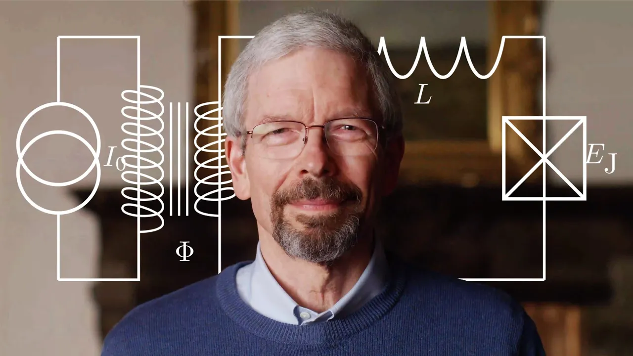
Superconducting Qubits Explained by Andreas Wallraff - QCHS 2021

[00:00:08]okay so welcome back everybody and now we are honored to have us next speaker professor andreas barath since 2012 andres varav is full professor for solicit physics at zurich after joining the deployment in 2006 as assistant professor previously he obtained a phd degree in physics from the university of erlangen and worked four years as research scientists at yale university during his career he has been awarded with many prizes to cite some economic school the european science prize in 2006 a european research council in 2009 max reussler price in 2011 and recently the helmholtz international fellow award 2020.

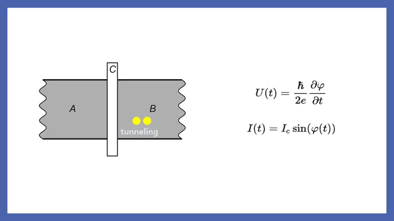
[00:00:47]in lecture today he will explain how these superconducting cubes that is this amazing i would say technology work so andreas thank you very much for joining the conference and i help you the stage all right thank you for uh for having me it's a pleasure to be here and talk at this school i even though it's not in person it's uh still one of the few schools that uh that i lectured in during the corona time so it's uh fun to be back here and hopefully we'll get a bit of interaction going uh throughout this lecture i i don't know how you are prepared for taking uh questions during the lectures as well or do you yeah actually if you want to compose at a certain point to ask to answer the question that haven't been asked or you can also answer hold the question at the end it's up to you and we can tell you which are the most interesting or more asked questions in case all right good so uh so i i would also plan to do maybe a short break uh somewhere in the middle of of the time that we have and we can also use that for um for questions also if you have any urgent questions just feel free to post them i guess in the chat and then the organizers can really relay those questions um to me good so let's see you still hear me my computer seems possibly to have an issue let's see whether i can so my slides don't advance now which is not good all right good so welcome once more to my lecture on on super conducting qubits i should acknowledge as at the get-go the contributions of everyone in our lab currently so i list both the phd students and postdocs on this title slide as well as our technical team and on the title slide you already see one of our super conducting devices and it's going to be one of the main actors of this lecture and on this particular seven qubit device we have realized the quantum error detection algorithm based on the surface code and i'll be aiming at explaining to you everything about superconducting qubits that you need to know so that you in the end you can understand how one would actually operate a quantum error detection algorithm in the surface code on this superconducting device and beyond the members in our current lab i should also acknowledge everyone who has contributed to our lab um throughout the years um and the both students and postdocs who worked with us are listed here and i also show where they currently are so i think there's an interesting mix between former lab members who are now a faculty at a number of places there's also quite a few who work for industry that relates to quantum like for example zurich instruments but there's also people working at startups like iqm and alice and bob and i also acknowledge our collaborators both at eth and elsewhere so maybe uh as a good starting point for this lecture we can take another look at this device which i showed to you already on my title slide a little bit uh so let me walk you a little bit through what you see here on this screen so the yellow objects are super conducting transmon style qubit there's seven of them they sit in this diamond double diamond like structure each one of the yellow qubits you can control with two control lines uh so the pink control lines here are used to apply um short say 10 nanosecond long microwave frequency pulses to the superconducting qubit to control its quantum state the green lines are used to apply short current pulses to the superconducting qubits and at the end of this line the waveguide is shorted so this current pulse will generate a magnetic field that will induce some flux through the loop through the squid loop of the superconducting qubit and that allows us to tune its transition frequency over several gigahertz in a few nanoseconds and this controllability is used to initiate two qubit gates in this architecture the qubits are coupled to each other through superconducting resonance structures so these are these turquoise transmission lines here that run from one qubit to the other in this double diamond structure and through those wave guides a capacitive coupling between the cubic qubits is mediated to initiate two qubit gates and then in addition maybe one of the special features of this chip which actually has enabled quite a few of the experiments that we've done on it in particular the quantum arrow detection experiments are these red and blue elements here which are lambda quarter coplanar waveguide resonators that are used for reading out the quantum state of the qubit so the red lambda quarter resonator is the resonator that is directly coupled to the qubit with a large coupling strength and has a strong coupling to the outside world so a large bandwidth or a large photon decay rate and this is then coupled to a another transmission line that is used for reading out the resonance frequency of this we read out resonator um through a so-called purcell filter which is yet another lambda quarter coplanar waveguide uh transmission line resonator and this per cell filter is needed to actually protect the qubit from spontaneous emission and one aspect that is also special about this device here is that you see that all these seven qubits they have all their individual readout resonators and purcell filters and uh in this device we can actually read out a group of four qubits through the same readout line and a group of three qubits through the same readout line so you see this uh dark purple wave guide here that couples first to the readout resonator of this qubit here and then to the readout resonator of the next qubit and to the readout resonators of this third qubit here and so essentially these resonators are staggered in frequency so that you can apply a single say multi-color microwave pulse to interrogate the microwave frequency resonators coupled to each individual qubit for reading them out essentially simultaneously in a frequency multiplexed fashion okay so now i think i have mentioned all the basic elements on this on this device here and we'll look a bit closer at them and as we go throughout this presentation good so my lecture is divided in these sections i'll give you a brief introduction to superconducting qubits and circuit qed then i'll move on to talk a bit about single and two qubit gates and how they are realized and these superconducting circuits and how we read out our superconducting qubits and in the final part of this lecture i'll apply everything we have looked at and learned to discuss this quantum error detection experiment which is a step towards realizing quantum error correction and superconducting circuits which is essential for realizing fault tolerant quantum information processes which is the target goal in quantum information science and in quantum in the realization of quantum computers okay so um that's about the schedule that we have ahead of us today and i plan to have a short break uh in the middle to take some extra questions and maybe for you to take a little break throughout this lecture good so let's start talking a little bit about superconducting qubits and how they're coupled to microwave frequency oscillators to realize this concept of circuit quantum electrodynamics um so you all know about conventional circuit elements electronic circuits are made from capacitors inductors possibly resistors and non-linear circuit elements such as diodes which you can then use to form transistors and these form the basis of all the communication and information processing technology that is based on say classical information processing ideas that we make use of every day and this has seen a long history from the invention of the full first non-linear semiconductor element the transistor at the bell labs that then got integrated to amazing integration depth with several billion of transistors on these centimeter size chips that we use today to process information also in my computer that just had my powerpoint file crash reason um so when you look at how to describe the physics of these electronic circuits while the materials properties need some quantum physics to understand them for example to understand how isolators and metals and semiconductors can be distinguished from each other all the information processing on these circuits is based on classical physics phenomena so quantum mechanics is not involved the superposition principle is usually not important and any of the control fields that we use are not not quantized and so maybe the first question that you ask yourself when you think about using superconducting circuits in the context of information science or in the context of doing quantum physics experiments is what how do you need to operate these basic circuit elements to observe the quantum mechanical properties so here i have probably an oversimplified example but i still like it as a as a starting point um so we are considering these basic elements capacitors inductors for example and we can see what charges and currents do on these circuit elements so one very simplified way to look at things is that you can consider such a capacitor here and if you consider a single electron we know that charge is quantized in form of electrons we could have the choice of putting that single electron on either one of these two capacitor plates and classically you have these two choices but quantum mechanically that single electron could be in a superposition of being on either one of the two capacitor plates and if one wanted to one could write this as this little pictorial wave function so that's in principle according to the microscopic quantum physics of particles like electrons this is in a large quantum mechanical state of an of an electronic circuit even though that under usual circumstances we rarely observe that in particular not at under room temperature conditions then you could also consider taking a an inductor and enclosing this inductor in a loop and you could consider a current flowing say clockwise through this loop here and classically you would imagine that that macroscopic current that is now made up of uh many millions of electrons would either flow clockwise in this loop or counter clockwise in this loop but quantum mechanically this current could be in a superposition of flowing clockwise and counterclockwise and in a pictorial wave function depiction you would maybe uh show this situation like that and that's already maybe a little less obvious that that could happen because now you're not talking about the quantum physics of a of an individual microscopic particle like the electron on the capacitor but you rather con consider the the quantum physics of a collection of electrons that behave coherently to form the superposition state of currents flowing clockwise and counterclockwise so maybe one of the most basic approaches to understand the quantum physics of these electronic circuits i think is to realize that charge and flux are a special variables to describe the uh the physics of these systems so the charge like the charge q that describes the charge on this capacitor or the magnetic flux phi that is generated by the current that flows through such a loop that current creates a magnetic field and that magnetic field creates a magnetic flux through the area of the loop and so charge and flux and electronic circuits have a special role they're conjugate variables like the position and the momentum are the two conjugate variables for a particle moving in free space and when you first learn about quantum physics you learn about the quantum physics of this free particles and how they interact with potentials and to to go from sort of a classical description of the motion of a free particle to a quantum description you promote these conjugate variables to quantum operators and you then have a promote your hamiltonian function to a hamiltonian operator and then if you have that hamiltonian operator you can start solving schrodinger's equation with it and make a quantum mechanical analysis of uh the problem that you're looking at and so essentially you can do the same thing that you've learned in your first quantum mechanics class for electronic circuits by making this realization that charge q and flux phi are the conjugate variables that describe the dynamic properties of the system so because these are conjugate variables there is an uncertainty relation that holds between them similar as the uncertainty relation that you know for position or momentum of a particle and and there's also a commutation relation between the operators that correspond to charge and flux so for example maybe i i spent a moment to now look at the the next more complicated example which is combining inductors and capacitors in this oscillator circuit so here you see a a combination of a linear inductor and a linear capacitor and when you create these circuits say on an integrated superconducting device you can choose capacitance and inductance values that make you end up with oscillators that have a frequency of a several gigahertz or so say five gigahertz in this case and on the side of this picture here i list a few typical circuit parameters for that so um an inductor like if you have a straight piece of wire it has an inductance of about a nano henry per millimeter so if you coil up a millimeter of wire on the circuit you get a nano henry of inductance and if you make a capacitor of about one picofarad the combination of that inductance and capacitance gives you roughly a resonant circuit with a five gigahertz resonance frequency and um so how do you think about the quantum physics of this circuit is you first start out with writing down the total energy for it and that's a combination of the magnetic energy stored in the inductor by currents flowing through this inductor and the electric energy stored on the capacitor so that's the flux squared divided by twice the capacitance is the magnetic twice the inductance is the magnetic energy and the charge square divided by twice the capacitance is the electric energy and now uh knowing that there is a commutation relation between flux and charge you can write down the operators for flux and charge and then replace these conjugate variables with a corresponding operators and then find this hamiltonian here which is quadratic and the two conjugate variables flux and charge which is characteristic for these harmonic oscillators and then you've solved harmonic oscillators many times in your quantum physics classes and you know that in second quantization it's hamiltonian can be written with these raising and lowering operators in the following form and the pre-factor of that is planck's constant times the resonance frequency of the harmonic oscillator and so this then allows you to see that this electronic circuit here is actually quantum mechanically described by a harmonic oscillator with a number of uh with an infinite number of states that you label from zero to n where the separation between the states is equidistant and given by planck's constant times the resonance frequency of the electronic circuit and sort of in in this way you can essentially go ahead and quantize uh any electronic circuit that you could um design or draw or make in your lab and uh here you can always really one way how we like to talk about these the excitations of these harmonic oscillators and microwave frequencies we like to think about them as storing microwave frequency photons all right so in which ways can you create these harmonic oscillators that i've discussed here there's actually quite a number of different approaches you could go ahead and realize this inductor capacitor combination that i've just shown on the last slide by making a long wire that coils up here and an interdigitated capacitor that you see on the on the right hand side here and this essentially realizes a combination capacitor you could also make these harmonic oscillators by just drilling a hole or making a cavity and a three-dimensional block of metal and this hole in this three-dimensional block of metal now supports electromagnetic modes it supports a number of these modes and but around the resonance frequency of each one of these modes you could describe that mode as a as a single harmonic oscillator or one aspect that we've you've seen already in my title slide and that we make of use a lot is you can make this coplanar waveguide resonators that cor that actually are made from a superconducting wire that is surrounded by a ground plane that then meanders across a chip between sort of an input coupler and an output coupler and that is also forming a harmonic oscillator with a number of resonant mode and modes and next to the resonance frequency of each of these resonance modes this is described by the hamiltonian that i've shown on the last slide or you could also consider say weekly unharmonic resonators if they're if the unharmonicity is weak enough you could also describe those in good approximation as harmonic oscillators so one of the aspects that is maybe a bit boring about these harmonic oscillators is that all their resonance frequencies uh or all their energy level separations are exactly equidistant and it's hard to address individual transitions between these different excitation levels of harmonic oscillators and therefore one would consider making these oscillators unharmonic so get rid of this linearity in the energy level spectrum and one of the ways how that's done in superconducting electronic circuits is to replace this linear inductor l here by essentially an ideal nonlinear inductor and this ideal nonlinear inductor is realized as a so-called joseon tunnel junction and in the linear inductor as we've just learned the magnetic energy is proportional to the square of the flux that is generated by the current flowing through that inductor in a joseon tunnel junction there is a current flowing through the joules in tunnel junction and that the magnetic energy that is created by that current is a cosinusoidal function of the flux that the current generates um so this cosinusoidal dependence on the magnetic flux is distinct from the quadratic dependence on the flux in this in this linear oscillator and this cosinusoidal dependence actually makes this oscillator then unharmonic through this non-linear inductor and i'll explain in a few uh in another slide a bit how this nonlinear inductor works um so this co-sinusoidal dependence of the magnetic energy on the flux then leads to an energy level spectrum in which the different energy levels are non-equidistantly spaced from each other in particular the ground to first excited state transition frequency is larger than the first to second excited state transition frequency which then again is larger than the second two third excited state transition frequency and there's one really very simple and intuitive way to see that so for example you can think of this harmonic oscillator circuit here as a particle moving in a potential and flux and charge are conjugate variables so you can choose a basis either the flux spaces or the charge bases and if you choose choose the flux basis then the potential energy term is quadratic in the flux variable that's just the magnetic energy and the particle is then a particle whose mass is determined by the capacitance of this capacitor and you could think of it as this particle moving in this quadratic potential and then if you quantize the motion of this virtual particle and this quadratic potential you find these equidistant energy levels so if you now replace your inductor by um by a joseon tunnel junction you get this cosinusoidal dependence on the flux variable and this cosinusoidal potential then opens up to higher energies in comparison to the quadratic potential and because the the potential energy landscape gets wider at higher energies or so the energy levels actually move closer to each other and then if you quantize this the motion of a particle moving in this cosinusoidal potential you will find exactly the situation that i've described on the previous slide that the first two that the ground to first excited state transition frequency is a little bit larger than the first to second and so forth and uh towards the top of this potential here the energy levels get closer and closer to each other and so this unharmonic superconducting circuit where the linear inductor is replaced by the strosin tunnel junction that then forms this unharmonic energy level spectrum in which we can now address transitions between the different states by irradiating it with microwave frequency radiation that is resonant with a specific transition so we can now through that radiation couple specifically the ground state to the first excited state for example by picking the right frequency and not coupling the first excited state to the second excited state simultaneously which would happen in a linear oscillator okay so um yeah since this is a lecture i think it's maybe good to uh to think briefly about where this cosinusoidal dependence on the magnetic flux in the joseon tunnel junction comes from so the jolts in tunnel junction which is symbolized in an electronic circuit by this box with a cross through it uh it's based on the joseon effect which brian josem discovered uh during his phd work uh at cambridge quite some time ago and so what he found when he analyzed his chosen tunnel junction which is a tunnel contact between two superconducting electrodes he derived a set of equations that describes the currents flowing through that junction and the voltage is appearing across it and actually it turns out there's uh two so-called josephine relations a dc and an ac jesus relation that are written down here so the dc josem relation says that the current flowing through the junction is the critical current times the sine of some phase difference delta across the junction and this phase difference delta that is indicated here so in the superconductor the electrons condense into a into a bose condensate of electrons in each of the two electrodes and as both condensate is described by a wave function whose pre-factor is proportional to the density of the electrons in the electrode and and the wave function has a phase factor that is where the phase vector is exactly given by this phases delta one and delta two and the phases of the wave functions and the two electrodes can be different from each other and what the dc joist relation says is that the current flowing through the junction is actually given by the sine of the phase difference of these wave functions then the ac joseon relation says that um that the voltage appearing across such a joseon tunnel junction is actually proportional to the time derivative of this phase difference delta and that proportionality is set or the proportionality constant is set by the so-called flux quantum so in superconducting circuits the magnetic flux is quantized and the quantization constant is finite which relates to planck's constants and twice the electron charge and so with these two joseon equations you can actually try to learn what the inductance of a joseon tunnel junction is and the inductance in any electronic circuit relates the voltage to the time derivative of the current and if you use these chosen equations to write down this relation uh you actually find that that the inductance has this specific form here namely is proportional to one over the cosine of this phase difference delta and this pre-factor is called this specific joseon inductance and it relates to this chosen flux quantum and the critical current across the junction and so now you can think of what is the magnetic energy stored in this junction and this magnetic energy can be found by integrating the product of the voltage and the current across the junction and there you find that this joseon energy is proportional to this pre-factor which is the product of the critical current times the flux quantum multiplied by the cosine of this phase difference delta and that's actually where this cosinusoidal dependence of the magnetic energy and the joseon tunnel junction comes from and then you can ask yourself okay what is this energy scale this chosen energy and it depends on this on the critical current of the joseon tunnel junction so the maximum current that can flow through it without any dissipation occurring and say if you would consider 100 nano amp nano ampere maximum current that would give you adjustable inductance of about three nano henries and that corresponds them to a jose energy of about 50 gigahertz or so so your co-sinusoidal potential is about 50 gigahertz deep so from the bottom to the top of the cosine is 50 gigahertz when the critical current of the junction is a hundred nano in pairs and so that's uh essentially what gives these uh superconducting electronic circuits their non-linearity good and the joseon tunnel junction itself i mentioned it already is made from these two superconducting electrodes that are separated from each other by a tunnel barrier and typical materials that are used are for example aluminum for the superconducting electrodes and aluminum oxide which forms a nice tunnel barrier that separates the two aluminum electrodes from each other and this typically gets then fabricated using electron beam lithography techniques in a clean room and here in this picture you see a horizontal superconducting strip a vertical superconducting strip and in this area where the two overlap they form a joules tunnel junction and the area of that tunnel junction is given geometrically and the critical current of the junction is essentially set by the density of the electrons and the two electrodes and the tunnel resistance across the junction which is given by the essentially the thickness of the tunnel barrier between the two electrodes and so this gets fabricated in a clean room typically in techniques that are known as shadow evaporation for example but there are also some alternatives good and with these elements with linear inductors and linear capacitors and these non-linear dosing junctions you can build many flavors of superconducting quantum bits here you see a selection of photographs of quantum bits that have been made from superconducting circuit elements maybe i'll i'll mention a few more explicitly so one of the very first ones that were investigated was this cooper per box qubit so that was work in a group of sierra sacre that that started more than 20 years ago now the currently probably most successful or most widely used super conducting qubit is the so-called transmon qubit um if you're interested in the details of that you could read this paper by jens cox from 2007 that introduced this qubit and it's really that or versions of it are are used in all the quantum computers at ibm at google and in most of the labs that work on superconducting quantum bits and there's variants of these trans ones like and you can one of the interesting names is that every time you come up one of the interesting aspects is that every time you come up with a different circuit you can give it a name and so i can play chemist from the early days when you if identified new elements you were free to give this new element a name and now when people actually invent new superconducting circuits they invent names for those so one of our graduate students already some time ago made this kind of interesting looking super conducting qubit and named it the jelly one and maybe interestingly at times there's heated discussions about what names are appropriate for these circuits so there was a in the community around superconducting circuits there were questions about how different the cooper bell box is from a transmon or an x-mon uh which uh interestingly all have exactly the same hamiltonian that describes its physics but the the circuit is actually used in slightly different parameter regimes and then has found these names that now are widely used good so um how does one operate these superconducting electronic circuits quantum mechanically so here's a one of these nonlinear oscillators that i mentioned the parallel combination of a joseon junction and a capacitor so that you then need to probe in some form and one of the ways to probe it is you could take a microwave frequency radiation source connect it through a coupling capacitor through this to this superconducting qubit and do a scattering experiment maybe similarly as you would take a laser and shine a laser on an atom and look at how the laser light scatters from the atom and the scattered light and superconducting electronic circuits you collect through by coupling another coupling capacitor to your qubit and maybe trying to um to uh guide the scattered microwave radiation towards a microwave frequency amplifier that then amplifies the signal which you can then digitize and see what you can learn about the circuit from from that digitized signal um so what do we need to do to observe the quantum properties of this superconducting qubit and so here's this my little three-step recipe so the first one is to avoid dissipation so using superconductors is good so because if you use normal metal components any currents flowing in these normal metal components will dissipate heat through the resistance of these components and this dissipation would lead to the energy relaxation from higher excited states back to the ground state by just leaving energy behind in these resistive components so therefore all the circuit elements need to be as lossless as possible so the second aspect that is important if you were to operate such a gigahertz frequency circuit so where the typical energy level separations are on on the scale of a few gigahertz or possibly a few tens of gigahertz if you would operate that at room temperature um room temperature is a much much higher energy scale than 10 gigahertz say so a good number to remember is a gigahertz of transitional frequency corresponds to 50 millikelvin of thermal energy so 10 gigahertz transition frequency qubit corresponds to sort of a 500 milli kelvin equivalent excitation energy and so if you take such a circuit and operate it at 300 kelvin even if you ignore the fact that it's not superconducting then yeah then it would be in a highly excited thermal state and therefore you just take your whole circuit and cool it down to temperatures which are much less than this typical energy scale of the transition frequency so we cool the circuits to 10 milli kelvin roughly and then uh the the other aspect that is important in circuit design and posed a challenge at least initially when these circuits were were designed is that you need to isolate the quantum circuit properly from your control and your readout electronics um and so you see that there is this coupling capacitor through which you couple the input radiation to your circuit and then there's a coupling capacitor through which you couple the detector to the circuit and um yeah if this coupling is too strong you could imagine that if you have an excitation in the superconducting electronic circuit that that excitation could actually leak back into the control electronics which is certainly undesired and it could leak back into the readout electronics and maybe the readout electronics leakages is good when you want to actually detect the state of the quantum circuit but in case you don't want to detect the state of the quantum circuit yet that leakage is of energy through these coupling capacitors is certainly not good and therefore you need to control the coupling strength for your control and readout electronics to the quantum part of the circuit well so that you can preserve the coherence of the quantum circuit good so so this is a slide that i wanted to show you later and that's probably got lost uh in my by in the crash of my powerpoint um so maybe the next step that is interesting to discuss briefly is the capabilities of that arise from combining linear oscillators with nonlinear oscillators and superconducting circuits [Music] and we've just discussed these linear oscillators that can be realized as discrete lc oscillators as coplanar waveguide transmission lines or as 3d cavities uh created by um yeah holes in metal blocks and superconducting qubits that are created by combining these nonlinear inductors with capacitors and possibly also with linear inductors and so there's an interesting concept that superconducting circuits inherited from um atomic physics and from essentially amo physics which is known as cavity qed and in cavity qed you investigate the interaction of say atoms or two level systems with optical frequency transitions and an electric dipole moment with optical frequency radiation that is contained say in a high quality mirror-based cavity and if your two-level system has a dipole moment that is of a significant size and the electric field generated by the photons stored in this cavity then the two level system can absorb individual photons from the cavity mode and coherently re-emit them into the cavity mode and this happens at a coupling rate that is known as g and this coupling ray g is proportional to the field strength created by individual photons inside the cavity and the dipole moment of the true level system and this is a convenient interaction or also a useful interaction because it allows one to convert quantum states stored in an atom into photons and the superconducting electronics version of that is shown here so there's a kind of this non-linear atom-like circuit and there's the linear cavity-like circuit and the two are coupled to each other through this electric coupling capacitor um and this coupling essentially creates the equivalent of the dipole interaction between the radiation field inside the cavity and the type of moment of the qubit and this is some piece of physics that has been investigated a lot in amo physics and sergia raj got a nobel prize for this a few years back um so why is this cavity qi qed idea so useful in quantum information processing so first it can be used to isolate qubits from the electromagnetic environment so when you take a say a superconducting qubit or an atom it doesn't really matter and if you detune its transition frequency from the cavity resonance frequency then you can actually suppress the vacuum fluctuations of the electromagnetic field present in the cavity two levels that are below the vacuum fluctuations of the electromagnetic field in free space and the strength of this electromagnetic field and its diplo pole coupling to any two level system actually sets the lifetime of the two level system and so if you suppress the vacuum fluctuations you will increase the lifetime so this can be done in cavity qed physics and actually the the very first cavity qed experiment ever observed that the lifetime of an atom was increased by bringing it in between two mirrors whose separation was small enough that the that the wavelength of the photon that the atom is trying to emit was longer than the separation between the two mirrors okay so this allows you deep bringing a detuned two-level system into a cavity allows you to enhance its lifetime and it allows you to do so while maintaining addressability of the qubits so you could still change the qubit state by injecting radiation into the cavity at the appropriate detuned frequency so one aspect about this combination of two level system and harmonic oscillator which is very useful is that it can be used to read out the state of the qubit and so i'll discuss that later in this lecture so when the qubit is detuned from the resonator actually the resonator inherits a frequency shift from the qubit that depends on the quantum mechanical state of the qubit so the resonator will have a frequency that is different depending on whether the qubit is in the ground or in the first excited state and that's something that is virtually used in all of the experiments on quantum physics with superconducting circuits then instead of coupling a single qubit to a harmonic oscillator you could decide to couple multiple qubits to the same oscillator and in this way different qubits could couple to each other by exchanging photons through this oscillator either virtually or exchanging real photons through the oscillator and then there's also this aspect that i've mentioned before you can use this coupling between the two level system and the cavity to convert the state stored in a stationary qubit into a photon and then you could emit the photon into a fiber and for example send that photon to another experimental setup and this also works for superconducting circuits if you couple a transmission line to this cavity mode you can actually launch a photon into that transmission line and send the photon elsewhere say to a different cryostat for example all right maybe a few more words on on cavity qed um so i've mentioned this basic aspect already uh so we we consider this atom inside the cavity and the interaction with the radiation field at this interaction rate g and there is a very simple hamiltonian that describes the physics of this system and this hamiltonian has just this harmonic oscillator part it has a two level part and then it has this interaction part where a dagger and a are the creation and annihilation operators of the radiation field inside the cavity and sigma minus and sigma plus are the operators that swap the qubit from the ground to its excited state and back and so this basic hamiltonian describes the physics of cavity qed and what one looks for essentially is the situation where this coupling strength g in this hamiltonian is much larger than any of the rates at which the coherence occurs here for example the rate at which you lose the photon from the cavity or the rate that you're uh two level system might decay into a mode not captured by the cavity so if you look at this hamiltonian there's a one way how to easily interpret the physics of it is to draw a so-called dress state's energy level diagram that is shown here and on the right-hand side a specific situation is considered namely the situation where the resonance frequency of the cavity omega r is chosen identical to the transition frequency of the two level system and so if that is the case a state where the cavity has one photon and the two level system is in the ground state or where the cavity has no photon and the two level system is in the excited state are at the same energy and if that's the case and the two are coupled by this dipole coupling strength this dipole coupling will hybridize these two states and lead to a splitting so that you essentially form a molecule between the photon and the cavity and the excitation in the qubit and this is known as the vacuum rubbing mode splitting and the size of the splitting allows you to directly measure this dipole coupling strength between the two elements and this dipole coupling strength for example limits how quickly you can exchange the excitations between the cavity field and the qubit and the holy grail of of cavity qed is to reach this limit where this dipole interaction strength is larger than any of this dissipative rates and this was something that uh it was an experiment that we did for the first time with superconducting circuits uh in 2006 uh when i was at yale working with uh rob shulkov and steve girvin and alexander blair on the theory side and and this coupling you can observe either spectroscopically by measuring this energy splitting or you can also measure it in a time resolved measurement by measuring these so-called vacuum radio oscillations and another important aspect that relates to this capability to read out superconducting qubits um actually considers this james cummings hamiltonian that i've mentioned in a situation where the cubit transition frequency is detuned from the cavity frequency such that the difference between the two frequencies much larger than the coupling string and then an interesting piece of physics happens that you can analyze when you look at this hamiltonian here so this is a hamiltonian which has been appropriately transformed to diagonalize it when the two systems are detuned from each other and what you see now is the term that has the a dagger a which essentially counts the photon in the resonator has a resonance frequency where the cavity resonance frequency is now cubit state dependent so it's changed by the amount coupling strength divided squared divided by detuning times sigma z which is the then the expectation value of the qubit state operator so if the qubit is in the ground state sigma z is plus one if it's in the excited state it's minus one and so therefore the resonance frequency of the cavity is shifted by either g squared over delta downwards or g squared over delta upwards dependent on the qubit state and this can be used to read out the qubit state and experimentally and actually it also performs a quantum non-demolition measurement of the qubit state because uh this hamiltonian commutes with a qubit state operator and so a pictorial way to look at that so you have the bare cavity at some resonance frequency if the qubit sits in the cavity at it in its ground state the resonance frequency will shift downwards if it sits there in its excited state the resonance frequency will shift upwards and now you can simply look at the transmission amplitude and decide by that transmission amplitude measurement whether the qubit is in the ground state or in the excited state good um so um maybe let me skip this slide and maybe finish this first part here with a few more general comments um so there's research on the superconducting circuits gets done and quite a number of academic labs i i think by now there must be more than 100 that master the capability of making these superconducting quantum electronic circuits and observe their quantum mechanical features uh what is maybe also interesting is that there is now lots of interest industry that is interested in using this technology to build quantum computers and not only large established industries like ibm and google but also startups like righty or iqm for example that that invest into this technology to master it for building quantum computers um so these devices that you've seen on this on this last slide here are our devices that are made at uh at these different companies and startups and maybe to give you an impression what things look like in our own lab so this here is a picture of a superconducting circuit that has 17 qubits mounted on it and sits in the sample holder here with 48 microwave frequency ports through which you can apply all the signals to this qubit that you need for changing its state for tuning its transition frequency for reading out the qubit states for example um this sample mount then or the sample then goes into a sample mount where it's protected from environmental radiation and shielded from magnetic fields so you see for example here's this aluminum cap which is good for magnetic field screening the whole assembly is in a radiation tight couple box and there's a 48 connectors leading to microwave cables that lead to room temperature then shielding these superconducting circuits from external magnetic fields is important so here you see new metal magnetic shields and an assembly of different parts that we use to mount the sample holder that you saw or the sample puck that you saw on the previous slide into a dilution refrigerator and here you see some of the assembly that includes this 48 port sample mount with several layers of magnetic shielding and then all the wiring that is needed to address all the qubits in such a setup and this whole thing then sits in a commercial dilution refrigerator um so this one here has been set up by uh by the people you see here johannes heinzo is now working for iqm and in finland and most everyone else is still in our lab at this stage and then once you've okay so on this on this picture here you see the sample mount sit at the bottom and then there's wires that go up through the different temperature stages to room temperature and there at room temperature you connect your wires to microwave frequency control electronics and together with this eth startup we're actually doing quite a bit of electronics development to have everything available that we need to run quantum experiments with several tenants of qubits so then if you have 17 qubits in your device or so your electronics starts to get a bit more involved and so this is kind of a scan across our current electronics setup and you see there start to be quite a few cables that you need to handle in controlling your your superconducting circuits good so i think this would conclude the the first part of my presentation and uh i think now what may be a good time to to possibly take a few questions and maybe take a break um also maybe depending a bit on on how much of the time we have to make up towards the towards the lunch break so maybe that's uh i would maybe take first a few questions and and then maybe with with uh uh um uber or francesco we can we can discuss how we do the timing for the rest of this lecture so yeah we have a question actually and the question is what is your approach to deal with the increasing complexity of the system with increasing number of qubits concrete how do you plan to reduce the number of inputs and outputs yeah that's an excellent question so so one of the measures that we have taken is we we for example on the readout side we're now multiplexing the readout so previously and in many experiments and also in quite a few of the experiments at ibm for example the qubits are read out individually so here we are now capable of reading out many qubits simultaneously through a single wire or through a pair of wires in indeed and multiplexing will be essential so at the moment we only multiplex on the qubit readout side but i think it would be interesting to think about how to multiplex on the qubit control side as well to reduce the wire count and this will certainly be an important question to address while scaling up system size okay we have another question actually do you plan to embed the superconducting circuit the whole circuit or even each one of the qubits into something like phonon band materials that could improve the coherence times okay so there's a question like how large is the interaction between the superconducting qubits and maybe a phononic degrees of freedom on these devices and and one needs to investigate the coupling mechanism there and so the the superconducting qubits store their quantum state in an electrical degree of freedom and this electrical degree of freedom creates electric and magnetic fields near the device and if it's mounted on a substrate that couples to these electric and magnetic fields for example because it's piezoelectric or it would launch say surface acoustic waves or bulk acoustic waves and uber can probably tell you a lot about that and and in our devices we actually try to avoid that um by using um materials that at least uh genuinely have weak coupling to electromagnetic fields but certainly if in the case that phonons start to play a role in these devices and normally they should be cooled down to very low temperatures because they sit in the same dilution refrigerator if those start to be a problem indeed doing photonic phononic band gap materials could be a relevant approach yeah that's a good suggestion okay thanks so there is a third interesting question so can you tell about any half force in the direction of coupling these superconducting qubits with either fine qubits in ions or atoms um yes uh so indeed a long time ago we we were working or thinking about doing something like that with uh with mood hefner for example on the iron side there's always been activities where one looks at hyperfine transitions which are also in the microwave frequency domain which could couple to these wave guides and there's a number of groups that that work on that and and we also do a few hybrid experiments ourselves and and these hybrid experiments are all very very challenging essentially because you add another technology that you need to master as well and and probably practically what has happened is that the progress on superconducting circuits was so fast that uh that the hybrid technologies uh really have a hard time sort of to to hold pace so i think while while what you suggest is really technically feasible um it's a big effort and one needs to make sure that that the hybrid system actually has improved properties relative to say the the clean simple system on which is based just on one technology i think it's certainly something to consider when it's needed but one needs to also make this hybrid technology be have properties that are at least as good as say the best property in your of the devices that you that you work with otherwise okay thanks so i will say last question and then we can take a five minutes break so that everybody can rest a bit so what would be the limitation in manufacturing qubits using high-temperature superconductors okay so that's a that's also an interesting question so what what role does temperature really play in these experiments and these cryogenic systems are um are commercial they're really a solid technology that now exists since many tens of years and moving to higher temperatures is really not that advantageous at this stage because cooling them down is not as difficult as as one might think so going to higher temperatures then would also require to keep the thermal excitation in these circuit elements low that would then mean so higher temperatures you could actually use high temperature superconductors so that the materials themselves stay but you still need to avoid thermal excitation so the transition frequency in the qubits would also need to be high in which case you then need um control electronics that rather than working say in the range of 5 to 20 gigahertz or so you would need control electronics that works at frequency ranges over several hundreds of gigahertz and and that is actually pretty impractical and and expensive and there's a less good technology um available there so that i think the the gain from working at higher temperatures um is is not high enough currently to to justify uh considering that okay so thank thank you and thanks everybody for the interesting question we can rest for five minutes and we meet again at 11 10.

[00:57:08]good and maybe i i would have still for you a question so what what uh ending time do we target now now we can also hand that uh 12 45 i think it will be good enough what do you think of that i wasn't that on the on the schedule it's at 12 45 yeah but uh we had some delay in the beginning right so maybe if you overshoot by ten minutes or something that's yeah yes okay so shortly before one would be okay you're saying yeah good so that i i think that should be fine i'll lm for that cool good forestry is very good andreas i notice you have a lot of really nice figures and pictures yeah is there someone in your group who is just really good at photoshop or do you uh use this eth service that no this is all i think this we all did ourselves more or less i think uh so i i i worked like between high school and university i i worked in in gr or in graphics a bit so i i did computer animations and things like that while at the end of my high school essentially in some technical documentation for for company for for some while in my uh and then i i kind of published a newspaper for hospital for a year or so and so i so you know a bit what to look for okay i kind some experience with these things and that's an interesting thing we'll mention next time in your cv introduction yeah yeah yeah definitely i i do like i do like this this was at the time so it's uh like a long time ago now when when desktop publishing and things like that were starting to be a thing yeah so before peop many of the things were done kind of manually and then people started to do uh animations computer-based and uh and also all this publishing business all turned digital and and sort of graphics based and i i i spent some time there and even uh uh i think at the time i also thought that one could have founded the company and that would have probably made some money initially uh like in the early days of that probably if it's like really growing field yeah i think it was clear i had good experience with that and was growing and i think that's there's certainly a niche until all the big uh publishers and and the advertisement houses and so on and learn the technology there is certainly a gap where you can kind of uh position yourself well i think and so i think that's where where my uh my interest uh comes from and having nice nice graphics and then there's there are certainly people in all others in our lab uh who have an interest on on that so i think this one here is from i think if salate put that together it's on the title of his phd thesis he's now at zurich instruments okay i would say we can start again actually there is another question i don't know if you want to answer it before sure okay so the question is why don't we use signals phase while performing the dispersive measurement generally first measurement give more accurate result than intensity measurement this is the question yeah so i'll i'll in one of the coming slides i'll say a few words about readout and maybe i can come back to that then okay good so then let's let's restart so in the first part i have told you about superconducting qubits and this com concept of circuit qed and uh how it's useful for quantum information processing and now in the remaining part of this lecture i'll tell you a little bit about single and two qubit gates and also qubit readout and then deploy that essentially to tell you a bit about quantum error detection in superconducting electronic circuits which is an experiment that we did about a a year and a half ago or so okay so here is my my one slide description on how to control single qubits i think this should all be quite familiar to you because it essentially works the same way as it works in any quantum mechanical two level system uh so you you identify the energy level spectrum of the system by doing some spectroscopy initially and then you can pick the transition frequency and then instead of switching on your microwave source continuously as in spectroscopy you apply a short microwave frequency pulse and then the com combination of the pulse amplitude and the pulse length will actually lead to a certain rotation angle of your qubit state and its qubit state space and here you see this block sphere representation of a single qubit state space and on the right hand side you see the real and imaginary part of the density matrix and the expectation values of the x y and z poly operators and what you see on this slide is all measured data so these density matrices and the expectation values of the poly operators are all measured and what is done in this experiment here is one applies a pulse with a certain phase and varies the amplitude or length to make this cubic state vector rotate about around this block sphere about two different axes namely about the x-axis and the y-axis and the qubit state is then identified by performing a measurement and how this measurement works i will i will say a bit more on later so here for example if you choose a certain pulse length you will do a quarter rotation around this the qubit block sphere in this case about the x-axis and then if you just double the length of the pulse or double the the amplitude of the pulse you will rotate it by exactly twice the angle and that cubit state vector will then go towards the south pole so now it's an equal superposition state on the equator and essentially what sets the axis about which one rotates this qubit state vector is the phase of the microwave frequency pulse that is applied to the qubit so here we chose one phase and then if you change the microwave phase by 90 degrees you will actually rotate about the y-axis instead and if you i don't know whether you watched it or not so um on the on the hand side you saw the density matrices changing uh in real time as the cubic state vector change and you also uh see kind of the um essentially the points to which the qubit state vector is pointing on this block sphere so now with this different phase angle on the microwave radiation that you applied to the qubit you now rotate about the y-axis instead of about the z-axis and as you see already in this demonstration data which is quite a few years old you can easily achieve quite high fidelities or quite high qualities for the qubit single qubit gate operations and now if you calibrate things properly you can have three nines fidelity and and there's even some groups and superconducting circuits that do it a bit better than three nines fidelity so this data was about uh uh two nines fidelity so an error less than one percent and in our lab we typically in the best experiments now we have on many different qubits we have errors typically below half a percent or so and and this is really the same technique that gets used for all two level systems uh when you when you control their state so in superconducting qubits there is a number of different ways how to enact two qubit gates and we use a particular version of that and i'll only discuss that rather than discussing maybe a range of different two qubit gates that one could realize and our two qubit gate is actually one that is initiated by tuning the qubit transition frequency in time and so here we see the states of two qubits qubits a and qubit b and so these state vectors 2 0 for example refer to the state of the left qubit and the state of the right qubit so our qubits as i said in the beginning because they have this cosinusoidal confinement potential they not only have two states but have higher excited state states as well and in this uh um experiment here in our way to realize this two qubit gate we use the second excited state of one of the qubits and here the qubit excitations are labeled 0 1 and 2 rather than g e and f and so what you also see is that here this state is the left qubit in its excited state and this right cubit in the ground state and the state here is the right qubit in its excited state and the left cubit in its ground state so you see that the two qubits are detuned from each other in this initial situation and then to actually perform the gate what it is that we do is we bring both qubits to the excited state to this one one state so we apply two pi pulses to each the left and the right qubit or single pi parts to each one of the two qubits and so that they're both in the in their first excited states and then actually to the left qubit we apply a magnetic field pulse that brings down the frequency of the left qubit and actually we bring the down that frequency such that this two zero state with the left qubit in the second excited state and the right qubit in the ground state becomes resonant with both qubits in the first excited state and so here's a little animation of that so we apply magnetic field to the left qubit and then also this one one stayed low as an energy because the one one state also has a left qubit component and we do that such that the two states are in resonance with each other and then since these two qubits are actually coupled to each other through a resonator like you've seen on my title slide and i as i've explained in the circuit qed context these two qubit states can now interact with each other and this interaction actually leads to a splitting or hybridization between this one one or two zeros state and this hybridization you can see as these two new states in frequency space and similar as i've mentioned for this time resolved vacuum robbie oscillations if you start not in an eigen state of this coupled system like in the 1 1 state then the system will oscillate between 1 1 and 2 0.

[01:08:03]so essentially the 1 1 state will go to 2 0 and if you double the interaction time it will actually come back to one one and the interesting bit is uh while you have cycled through this interaction exactly once you're you're back in the in the initial state but since this is a quantum mechanical system this uh upon this transformation you have picked up a minus one phase factor in front of your one one state and now you could also look at what would have happened if you had started in the zero zero zero one or one zero state and if that would have been the case yeah then um then none of these other states would have interacted with anything else so they would have just stayed where they are and what that means is is that that those states would have remained the same even when you detune the qubits back to their original transition frequency and so the the three other states 0 1 1 0 and 0 0 require no phase vector while the 1 1 state acquires a phase vector and this actually one uses to create a so-called controlled phase gate and the unitary that belongs to that is the unitary that is shown here which has ones on the diagonal and a minus one in the last entry that describes this phase change for the 1 1 state and together with single qubit gates this c phase gate can actually be turned into a c naught gate and therefore is one of the components for performing universal quantum computation so this is a universal two qubit gate and so this c phase gate is typically depicted by the qubit lines run horizontally and when you do a c phase gate between the two qubits it's indicated as these two bullets linked to each other by a line and to turn that c phase gate into a c naught gate you to one of the qubits you apply two single qubit rotations and here in this notation here r stands for rotation single qubit rotation y indicates the axis about which is rotated and pi half says the angle about which it is rotated and if you do this two single qubit operations this actually turns the c phase gate into a c not gate and this will use later in this error correction experiment or error detection experiment um so what can you do to verify that this actually happens in this experiment so what we do in the experiment we bring both qubits to the excited state then we apply magnetic flux to one of the qubits to bring it into resonance with the other one reduce the flux again and look at the final state and to see that this c phase gate works one of the characterization measurements that one can run is the so-called process tomography and in process tomography you ask yourself if you have some process e applied to some initial state characterized by some density matrix rho what will be the resulting density matrix after you applied that process and one of the ways how to determine that is to actually decompose this generic process e into an operator basis e k and this operator basis for every individual qubit is just the identity matrix and the three poly operators x y and z and you can essentially decompose any arbitrary process acting on n qubits into an operator basis express process that combines identity and poly operators on each one of the individual qubits and the element that then describes that process is the the so-called chi matrix here are the process matrix and this process matrix defines or describes the weights with which these operators act on this initial density matrix row to produce the final density matrix rho prime and to actually measure this process matrix chi you feed all possible single qubit states to the input of that process and do tomography at the output of the process and from that you can then with some linear linear algebra reconstruct the sky matrix for example for the c phase gate which we've done here and the gate fidelity for this example was 99 or so and in our lab um typically we can do gates with fidelities around 99 but in larger devices at times the fidelity is also a couple of percent lower than that and as i said already before you can turn the c phase gate by this two extra single qubit rotations into a c naught gate which is then the archetypal gate that two qubit interactions are expressed in the quantum information process good so uh that's all i wanted to say about two qubit gates in superconducting circuits in particular picking the example that we use in our own lab and that's also like widely used by other labs but there's also many other two qubit gate realizations that get implemented by other academic and industrial groups in the field so i want to say a few more words about qubit readout where before i then switch to the final topic of how to do error correction in or error detection and superconducting circuits so here you see a um a little patch of the device that i we discussed already in the beginning so there's a superconducting qubit shown in yellow um it has this uh um microwave frequency control line in green for applying single qubit pulses oh sorry that's that's wrong so the green line is the the flux line that tunes the cubic transition frequency and this uh pink line is the one through which we apply microwave frequency pulses and then the readout gets done by coupling a microwave frequency resonator to this yellow qubit and that's this reddish lambda quarter resonator that has an open end on the qubit side and is shorted on the other side and this lambda quarter resonator acts as the as that resonator the frequency shift of which we measure to determine the qubit state and then that's not directly coupled to an input line but coupled through this purcell filter here which you see looks essentially the same it's a it's another microwave frequency lambda quarter resonator tuned to the same frequency as the readout resonator frequency and the two are coupled to each other and the combination of the two is coupled to some feed line uh here and actually the sort of the white strips that you see here are air bridges so in on this chip there is a um [Music] we can realize some crossovers and connections between the ground planes using these air bridges i need a cup of water maybe i can take a question while i drink some water or there are no questions in the chat but uh we are encouraged to ask questions if you have something that i would like to know or something that didn't understand well [Music] okay there's no further question i had my glass of water let's hope that might have a question that was asked so maybe we can answer so why is the qsh0 say to be an electronic photon on these lights photons don't have any energy levels this is the question i think you're muted i don't can't see if you're okay yeah that that i didn't notice sorry um now i'm coughing again sorry if you want you can take another cluster of water we can have another break no that that's fine so okay so i was um so so these resonators they can uh you can actually um load them with individual photons if you want to it has an um a linear energy level spectrum the ground state has no photons and then you can add photons one by one for example by loading them through the qubit through interactions with the qubits or you could also put coherence states into these resonators for example by taking a coherent radiation source that you apply through this input port to this resonator and then actually for all these readout experiments we we use coherent tones and coherent tones are bosonian distributions of photon numbers with a with a given phase that populate the resonator with an electric field with a with the minimum uncertainty amplitude and phase as allowed by quantum physics for the coherent states i hope that at least did catch the right direction of the question so i said that there is this red part as the readout resonator the blue part is the purcell filter um the special thing about this chip was that there's multiple of these resonators coupled to a single readout line so that we can frequency multiplex [Music] what is also special is that there's a large coupling between um the qubit and the readout resonator and this large coupling leads to a large dispersive frequency shift um that means that the resonator shifts a lot in frequency when the qubit changes state and that's convenient for um doing high fidelity readout all right excuse me good and another important aspect in this readout is you need to be able to detect the microwave radiation that gets scattered of these radar resonators effectively and in superconducting circuits we do that using parametric amplifiers and these parametric and these parametric amplifiers they they can detect microwave frequency radiation uh close to the limits that are allowed by by quantum physics so they can add very little noise to the signal and then enable a high fidelity detection of the cubed state so here you actually see an example of what i've explained previously so this is a transmission spectrum of the readout resonator with its per cell filter so if there was only a readout resonator you would see a single lorentzian line but now we have a essentially two lambda quarter resonators coupled to each other and the coupling combination which you choose leads actually to the spectrum where you have kind of a broad envelope and a dip in the middle of it and this comes from the interference between um the radiation the radiation interacting with this per cell filter readout resonator combination and we measure that spectrum then once for the for the qubit being in the ground state and once for the qubit in excited state and what you clearly see is that the spectrum is shifted in frequency by a fair bit so this axis here is uh scaled in gigahertz and the frequency shift between the two states is roughly 16 megahertz or so and the the width of these lines actually tells you about the the bandwidth of this readout resonator and the wider these lines are the faster you can get photons into the readout resonator and out of it again and this combination of purcell filter and readout resonator is used to have large photon decay rates while not affecting the qubit lifetime too much okay and then so essentially you can then choose an operating point you choose some frequency and then you measure the transmission through the resonator depending on whether the qubit is in the ground state or an excited state and here you see transmission amplitude so it's not decomposed into two quadrature amplitudes there was this question before that was asked whether you should measure amplitude or phase or power for example or any of the quadratures and effectively in our experiment we measure two quadratures and but in this plot here there's the transmission spectrum shown in amplitude so if you want to do a good readout when you look at the amplitude you would pick a frequency at which the two amplitudes are as different as possible and so for this demonstration experiment we have then done that so here you see what is plotted on this on this graph here is what happens when you apply a readout pulse to this readout resonator this readout pulse starts at the time t equals zero and then the resonator gets populated and we measure a transmission amplitude through that resonator and how it depends on time once for the qubit being in the ground state um and and then also for the qubit being in the excited state and sort of a single measurement trace actually looks like this a wiggly curve with a dots that are connected by straight lines and then if you repeat that experiment a couple of thousand times and average you find the average light blue curve and the standard deviation of the distribution at every point in time is indicated by um by the the white band that you see in the background but you clearly see that that each individual curve um for the qubit in the ground state uh looks roughly like that and when you compare it for example to an excited state each individual excited state curve looks distinctly different from the ground state curve yeah so and that comes from the resonator frequency shift that is induced by the qubit state change and here again like the red data set is an individual measurement so where you prepare the cubit once in the excited state you switch on your measurement once you digitize the measurement data and the solid line is one where we averaged over a few thousand traces and the standard deviation is shown again by this orange white band in the background and then to actually determine the qubit state what you do is you integrate that detection signal over time over a given time window that is indicated by tau and where tau measures the time from the moment that you switched on your readout tone until you stop considering the data and now you see the two data sets again and you clearly see that both for individual traces and on average you can clearly distinguish ground states from excited states and the typical characterization measurement that you then frequently do is you you pick an integration time tau say 50 nanoseconds or 100 nanoseconds and you integrate the readout signal over that time and then you put that value into a histogram and you condition the histogram on whether the qubit was prepared in the ground or in the excited state and you look at what that histogram looks like and on this slide you see such a histogram so here's the integrated measurement signal on the on the x-axis you've seen every time that the qubit is in the ground state um the integrated measurement signal is negative and the distribution of the integrated measurement values is shown by this histogram here and you see that it's roughly gaussian and there's a distinct other distribution for when the qubit is in the excited state it's also gaussian and the two distributions are shifted from each other and for the excited state you also see that even at this short integration time of 56 nanoseconds there's some finite probability that the qubit will have detected to the will have decayed to the ground state before you've finished your integration time and mind that this is a logarithmic scale here so there's very few counts um at in this part of the histogram here which identifies the states or the instances where the qubit had already decayed to the ground state while it was prepared in the excited state and then measured and the quality of the measurement you can now actually characterize in different ways and one of the ways is to consider the overlap error error in these histograms and the overlap arrow is actually one that the that reduces as you increase the uh integration time so when you increase integration time essentially the the resin the histograms move apart from each other and the overlap error gets reduced but as you increase the integration time then the qubit when it was in the excited state has more opportunity to decay and therefore the the error in the state identification due to qubit decay increases and there's also another error source namely that there is a small probability that the measurement itself might change the qubit state as well and so one of the things that we've looked at we've checked both versus integration time and versus measurement field strength how the measurement error actually varies um across these parameters and here's the data set that shows measurement integration time shows the measurement error versus measurement integration time and when the measurement integration time is very small the measurement error is large and as you integrate more the two readout signals they separate from each other you saw in this plots in this plot on two slides ago that the ground state trace that go to low values and the excited state trays that go to high values and they get more and more distinguishable the longer you integrate and then there is an optimal integration time scale beyond which then you start to get errors that stem from the qubit decaying from the excited state to the ground state and at that integration time you then get optimal fidelity and for the example that you see here you get a fidelity of about 99 in in about 15 nanoseconds or so okay so so this uh kind of concludes this single qubit gate two qubit gate and and readout part and i have a couple of slides that i don't think that i have time to discuss but i'll just leave here for a second you can hold it up later so this these slides show you some examples of recent work in quantum information processing with superconducting circuits um so there's lots of basic works has been done in the in the past 15 years for demonstrating all the elements and currently um in quantum information processing the work is focusing on implementing schemes for error correction and also implementing so-called nisk based approaches so implementing algorithms that might result in sort of interesting outcomes without requiring a quantum error correction to be implemented and so those fall into different categories namely you could perform digital and analog quantum simulations with these mid scale superconducting circuits and a particular example of that is for example work on quantum chemistry so there's quite a bit of interesting um experimental efforts that use mid-scale superconducting circuit devices say with several tens of qubits to perform quantum chemistry simulations essentially calculate ground state and also excited state energies of small molecules and kind of try to point at how that could be a useful approach for quantum simulation with superconducting circuits and and also with other quantum information processing systems and maybe a third application area is using small scale superconducting circuits for quantum approximate optimization algorithms where you find an optimal solution by running a quantum algorithm on a superconducting circuit and here's a few examples of those and also our own lab has worked on that a little bit good so um in the last 20 minutes or so that i have um or i know it's more 15 that i have i'll i'll tell you a little bit about quantum error detection and error correction so you probably all have heard about this quantum computational supremacy experiment by google that was now done uh maybe close to two years ago and it used 53 qubits on a 54 cubit chip everything was working really quite nicely on their chips so they had two qubit operations with less than a percent gate error they had even better uh single qubit operations on this device that were significantly less than a percent error their their readout on this device was was good maybe not quite as good as the readout that i presented in the in the last slide but they had a much more complicated device with many more qubits to read out and what they've implemented on this device was kind of essentially a randomly chosen gate set that would create a very complicated entangled multi-particle qubit state at the end of this random gate sequence and then they try to simulate that random gate sequence outcome on a classical computer and showed that that's very hard to do on a reasonable time scale so in that sense the quantum computer outperformed the classical computer in creating a proper quantum state at the output which had the desired statistical properties but one of the aspects that is important to point out in this quantum supremacy experiment um the fidelity with which the final state of this 50 qubit processor corresponded to the one that you were expecting uh was only about 10 to the minus three so the the final state is not very close to the to the ideally expected state and this indicates that in the end you need to be able to correct for errors that occur both errors that are induced by the gates themselves and also the coherence errors in these circuits and one of the ways to do that is to make the quantum computer fault tolerant through quantum error correction and quantum error correction i'll essentially spend a few minutes to explain the concept so rather than encoding your quantum information directly in physical qubits um where every single qubit actually stores one quantum bit of information in error correction you you try to at least in the surface code version of error correction you distribute the quantum information across a larger number of so-called data qubits and then you try to measure properties of these data qubits using so-called ancillar qubits without destroying the quantum state of the data qubits and one of the approaches called the surface code is shown here so there's this square array of data qubits shown in red so it's a five by five so 25 qubit array of data qubits and you try to store your quantum information in sort of a complicated entangled state of these data qubits and then these data qubits are interspersed by so-called ancillar qubits that couple to four nearest neighbors and these ancillar qubits can be used to measure certain symmetry properties of the data qubit states and i'll explain that in more detail in a second so this here this device or this layout that you see has 49 qubits and for the experts among you that that would be a plus it would be big enough to realize a distance a 5 surface code let me say a bit more about these data qubits and and the ancillar cubes and what they're used for um so the ancillary qubits come in these two types so called x and z ancillars and these x and z and they measure different symmetry properties of the quantum states stored in the four neighboring data qubits and using these ancillary qubits you perform so-called stabilizer measurements so you measure these combinations of four z operators and a weight four stabilizer or two z operators and a weight two stabilizer um along the z axis or you can do the same thing in the x-axis so you measure the expectation value essentially of the combination of the x operators x1 x2 x3 x4 where the different the the indices one two three relate to the coupling of this ancillary qubit here to the four uh nearest neighbors data qubits and at the edges uh there's ancillar qubits that measure this the parity or the stabilizer when they couple to just two neighboring qubits and how do these stabilizer measurements work in these stabilizer measurements you essentially perform c naught gates between each data qubit and one of these ancillar qubits and since in our circuits we don't realize c not gates directly but the c phase gates which i've explained to you before here the two qubit gates are indicated as the c phase gates with a uh indicated by these lines that connect the data qubit with the ancillar qubit and to effectively turn these four c phase gates into four c not gates we use single qubit gates in addition and you see that the single qubit gates that sit in between the two qubit gates they they just cancel each other out because they all act on the same ancillar qubit and and what this gate sequence here does i'll explain it at a more simple example on the next slide so this this circuit here performs the so-called z-stabilizer measurement and if you uh flip the bases of the data qubits by applying pi half pulses to them and then apply the same gate sequence you can also measure the data qubits in the x spaces and thereby perform an x basis stabilizer measurement and for that to work well you see that you need to apply quite a number of two qubit gates and also single qubit gates which all have to happen in high fidelity because this error correction code relies on being able to measure the symmetry or the parity of this four qubit stabilizers with with high with high fidelity so that you can actually tell whether an error occurred or not okay and and this uh whether an error occurred or not you can actually find out by after this gate sequence performing a measurement um on the ancillar qubit so in this error correction scheme you need to be able to run these gates very effectively with high fidelity and also be able to measure the ancillary qubits without disturbing any of the data qubits so let's maybe explain how this parity or stabilizer measurement works on the in a way 2 stabilizer example that is simple so here you would measure the z1 z2 stabilizer for two data qubits and you essentially apply a c not gate between each one of the data qubits and the ancilla and now if the c not qubit the c naught gate it does nothing when the qubit is in state zero yeah so essentially in for the zero zero data qubit combination the ancillary qubit just stays in its ground state where it's been initialized initially when both qubits are in the excited state the two c not gates will subsequently flip the ancillar qubit first from the ground to the first excited state and then back from the first excited state to the ground state so when you have an even number of ones or an even number of zeros in your data qubits yeah the ancillary qubit will remain in the ground state and that indicates an even parity data qubit state so an even parity says that both qubits are in the same state so either both zero or both one well when the data qubits are in an odd parity state say one of the qubits is in the in the ground state and the other one is in the excited state then one of the c not gates will flip the ancillar qubit from the ground state to the excited state and now your insular qubit tells you that your data qubits are in odd parity state and so now the whole idea of the surface code is to to encode quantum information in states with a given parity so you would decide for example to encode quantum information only in states with even parity say where there's the same numbers of zeros and ones and if that's the case then um the ancillar qubits always stay in the ground state and if then an arrow occurs yeah one of the qubits will flip from either the excited state to the ground state or from the ground to the excited state your ancillar qubit will tell you that the parity changed from even to odd and this parity change you used to actually identify whether an error occurred or not and the interesting thing is in the surface code you can do that without learning uh the state of the logical qubit that you have encoded in your data qubits and that's what i explain a bit more on the next slide so here's the on the surface code here we don't implement a distance 5 surface code on these 49 qubits but the first thing that we did in our lab is we implemented the distance 2 surface code on just seven qubits uh that you see here and um so there's four data qubits and three on silver qubits and uh um so as you see here there's one blue ancillar qubit that measures the x parity and two green ancillar qubits that measure the way two z parities and the interesting bit is that this set of stabilizers they commute with each other so these three operators commute with each other and therefore they have joint eigenstates and for example in these joint eigenstates you can then encode the logical qubit and so you could encode the ground state in this combinations of zeros and ones of the four data qubits and the excited state in this combinations of zeros and ones and you see that both of these states have both even parity and now for example if one of the qubits would flip state then that would be indicated by an ancillar based parity measurement as a state change in the ancillar qubit and that allows you to identify whether an error occurred and logical superposition states are then superpositions of these basis states and they obey the same properties and so you're allowed on these states to measure their parity without actually learning which state your logical qubit is in and that's the whole key idea of of quantum error correction that you can perform measurements to identify whether errors have occurred without learning the quantum state that you've stored in this logical qubit and this is really the simplest example that you can realize there and then you can perform logical operations on these qubits by uh actually applying um logical operators on them so to perform to flip the logical qubit state you can perform this x1 x3 operator on the zero state and that will actually flip the second and the um will flip the first and the third qubit from the ground to the excited state and thus turn a uh a qubit excited state into qubit ground state and these logical operators then anti-commute with the stabilizers and that's that's what you want anti-commute with each other all right and so i i have virtually no time left and so i can maybe only give you the idea of the experiment so here's the device that i've explained to you in the beginning with its seven qubits and you now should be knowing what all these different elements on this circuit are are used for so here you see how you would identify the four data qubits d1 to b4 and three ancillar qubits um here's set of some parameters about the performance of these qubits like their lifetimes and their transition frequencies and how well we can read them out and essentially we can perform very good single qubit rotations on every one of those qubits with much less than a percent error and on this device the two qubit operations were actually worse than what i've explained to you before they're somewhere on the um say two to four percent level but overall this device was good enough to actually implement this distance to error detection algorithm and uh and this was actually the first time that the surface code distance to error detection was implemented in any superconducting circuit device and obviously this is based uh on quite a bit of prior work that was done in other labs and also in an industry on error detection and error correction so we used elements uh that have been tried out before but this uh for quite some time for about a year was the sort of the best error correction and detection experiment and superconducting circuits and by now leo de carlo's lab and both ibm and google have equivalent experiments that realize this distance to error detection circuit okay and um so i think now we're essentially out of time and uh i've been able to explain to you the idea of the surface code distance to error detection and now i should probably ask uber uh how we proceed here i could just wrap it up and take a few more questions and then let people go for for their lunch that's a good idea we have actually three questions in the chat here and there were a few more on the youtube stream so we have ample questions to fill a few okay good we could do that i should probably also say is um that i've i've presented this uh um the work on the error detection at a number of other occasions and maybe we can put a link for that so those of you are interested in the details um could could look at that and i could take a few more questions uh if you have this the remaining slides available we can also distribute them yeah i could do that so if you just send it to us we'll yeah upload them cool francesco no i want to account sorry but okay the first question is in the readout is there one error type preferred over the other maybe because of it applies to both the set equally yes so there's i think the the decay arrow is more prominent because uh the qubit will decay from the excited state to the ground state and so that that error source occurs more often and the ground state unless there is thermal excitation or measurement induced mixing should the ground state error should occur with a smaller probability so in in many instances the residual error is is limited by excited state decay at a given integration time okay so another question how to make sure that performing c naught gates between two qubits doesn't couple other qubits that are not meant to be used that that's a very important question um we've we've looked at that um a fair bit so one of the aspects that you need to make sure is that there's no unwanted interactions with the neighboring qubits and so you have to arrange them in frequency space such that no interactions occur so in particular in the surface code letters that you've seen a single ancillar qubit couples to four neighbors and you have to stagger the data qubits and the ancillary qubits in in frequency space in a way that you can target a certain coupling and have preferably no or only very small residual couplings to to other neighboring qubits but this residual qubit coupling is actually a challenge and and we've addressed it also in in a paper where we've analyzed that a bit and it's sometimes discussed in the terms of the role of spectator qubits in in these larger devices okay then they want to know if bosonic codes can be implemented in your experimental setups okay so one thing that i i really didn't have time to explain in um in more detail i haven't even mentioned at all is that this surface code error detection is a qubit-based uh or a service called error correction it's a qubit-based error correction code um you can also consider error correction codes based on bosonic systems and those can be realized for example in the oscillator modes of ions or in in resonator oscillator modes in in these superconducting circuit devices and this is also very successfully done and maybe in terms of performance of the logical qubit this is even a bit ahead of on the surface code implementations and one of the labs that really does pioneering work there is the other groups of rob schilkov and michel devery at yale for example so you could look at their um at their work there and i think i also had a few citations on one of my slides on that positive code work okay and then a question on error correction they want to know if there are alternatives to the surface code that require less ancillar qubit for each uh let's say a logical qubit i think there's a wide range of different codes that could be used uh the the surface code stands out as one that has the highest error threshold yeah so in the end what you need to achieve is that um say the the signal and two qubit gate fidelities and also the readout fidelities and all our other errors need to be lower than a certain threshold so that the logical qubit actually performs better than the physical qubits and that's very demanding and the surface code is the one which has is most tolerant to errors occurring and and other codes are are typically less tolerant uh um to errors occurring and so have even more stringent requirements um on the on the gate and readout errors but there's lots of literature on different codes and exploring different codes and maybe looking at codes that are more targeted towards certain era sources is also an interesting subject of research okay then things are quite advanced in time i would ask a last question it comes from youtube so the question is does the implementation of this c phase use an ac or dc pulse and thus these implementation also cause leakage defects yes so this the c phase gate that i've discussed is uh based on on a dc pulse and and indeed there is the possibility of leakage occurring in these gates in particular because the you use the second excited state of one of the qubits yeah and for example if you don't manage to remove all the excitation from this qubit that cycles through its second excited state that can lead to leakage and that needs to be suppressed and it's one of the the error sources in this two qubit gate which is particularly detrimental for example in error correction settings where like leakage errors are particularly difficult to recover from so that's a good question i think uh we are done thank you very much for the talk that i would say resonates very well with the spirit of our school and so now we can have lunch there is one hour approximately of lunch break we will be back at two there is the torque of dario gil uh from ibm remind that the link is not the same of this uh webinar is another web link webinar and you can find it on the leaflet of the school so we'll get two on the other link and then there is the tutorial all right thank you very much thanks for having me uh sorry for the technical problems in the beginning and also the technical problems with my voice and being out of time a little bit but i hope you still got something valuable out of this contribution thank you thanks a lot absolutely thank you very much that's a great talk thanks so do i send you the slide set or um yeah if you just uh send them to me by email and then after it's full then we also send the link for the recordings um we'll just include the slides i think uh vincenzo also already send us his slides and we'll just keep collecting while we go in the next week or so we distribute them all right yeah thanks a lot sorry for the technical difficulties yeah absolutely no problem we have large breaks in between all right thanks bye