The Chelyabinsk meteor explosion on February 15, 2013, demonstrated how meteor debris can be transported globally through the atmosphere; scientists used the OMPS instrument on the Suomi/NPP satellite to track the plume's journey, revealing that differential wind velocities at different altitudes caused the debris to form a complete global belt within four days, with the stratosphere acting as a transport pathway rather than a barrier.
Chelyabinsk Meteor Plume: NPP Satellite & OMPS Data Analysis
Added:Deep Dive
Understanding the thermal and physical structure of Earth's atmospheric layers, particularly the stratosphere and troposphere.

IAS 2021 | Gurukul 2.0 | Geography by Sumit Rathi | Structure of Atmosphere | Part-3
45.5K
The atmosphere is divided into layers based on temperature and composition. Thermal structure: Troposphere (0-10 km) has decreasing temperature with altitude; Stratosphere (10-50 km) has increasing temperature due to ozone absorbing UV radiation; Mesosphere (50-80 km) reaches -100°C (coldest); Thermosphere (80-450 km) reaches 1200°C due to oxygen absorbing UV; Exosphere (450 km+) merges with space. Compositional structure: Homosphere (0-88 km) has well-mixed gases; Heterosphere (88 km+) has gases separated by molecular weight (N2, O2, He, H). The Troposphere contains 75% of atmospheric gases and all weather activities. The Stratosphere contains the ozone layer (O3) that absorbs harmful UV radiation, making it the 'life-saving layer' that enables life on Earth.
Click to watch →
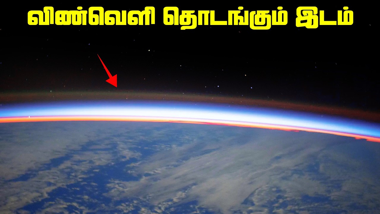
விண்வெளி தொடங்கும் இடம் - Atmosphere Layers
82.2K
Earth's atmosphere is divided into five layers based on temperature variations. The troposphere (0-12 km) contains 75% of atmospheric gases and all weather phenomena, with temperature decreasing from 15°C to -52°C. The stratosphere (12-50 km) contains the ozone layer that absorbs 90% of harmful UV radiation, causing temperature to increase from -52°C to -15°C. These layers are separated by the tropopause, where temperature inversion prevents air mixing. Commercial aircraft fly in the stratosphere for stable conditions.
Click to watch →
![ବାୟୁମଣ୍ଡଳ ର ବିଭିନ୍ନ ସ୍ଥର। Layers od atmosphere [in ODIA] | troposphere, stratosphere | Bayumandala](https://i.ytimg.com/vi_webp/2khT5ilNg9Q/maxresdefault.webp)
ବାୟୁମଣ୍ଡଳ ର ବିଭିନ୍ନ ସ୍ଥର। Layers od atmosphere [in ODIA] | troposphere, stratosphere | Bayumandala
58.8K
The troposphere is the lowest layer of Earth's atmosphere, extending from the surface to about 10-12 kilometers altitude. It contains most of the atmosphere's mass and is where weather phenomena occur. The stratosphere lies above the troposphere, extending from approximately 10-12 kilometers to about 50 kilometers altitude. This layer contains the ozone layer, which absorbs harmful ultraviolet radiation from the sun, protecting life on Earth from radiation damage.
Click to watch →

المحاضرة الأولى فى الباب الثانى - علوم مُتكاملة - مكونات وطبقات الغلاف الجوى - أولى ثانوى
237.3K
Earth's atmosphere is divided into five layers: (1) Troposphere (0-10 km) - where all weather occurs, temperature decreases 6.5°C/km, contains most water vapor and living organisms; (2) Stratosphere (10-50 km) - contains ozone layer (20-40 km) that absorbs harmful UV radiation, temperature increases due to ozone absorption; (3) Mesosphere (50-80 km) - coldest layer at -93°C, where meteors burn up; (4) Thermosphere (80-700 km) - reaches 2000°C due to absorption of high-energy solar radiation; (5) Exosphere (700-10,000 km) - outermost layer where satellites orbit and some gases escape into space. The tropopause (10-11 km) marks the boundary between troposphere and stratosphere.
Click to watch →

বিসিএস সাধারণ জ্ঞান প্রস্তুতি | বায়ুমণ্ডল | ৩ মাসে বিসিএস প্রস্তুতি | 45th bcs | bcs online tutor
73.4K
The troposphere extends from Earth's surface to approximately 14.5 kilometers altitude, where temperature decreases with height. The stratosphere lies above, extending to about 50 kilometers, where temperature increases with altitude due to ozone absorbing ultraviolet radiation. These two layers form the lower atmosphere, with the troposphere containing most weather phenomena and the stratosphere providing protection from harmful solar radiation.
Click to watch →
Deep Dive
Basic principles of satellite remote sensing, including how sensors detect atmospheric aerosols and trace gases through spectral observations.
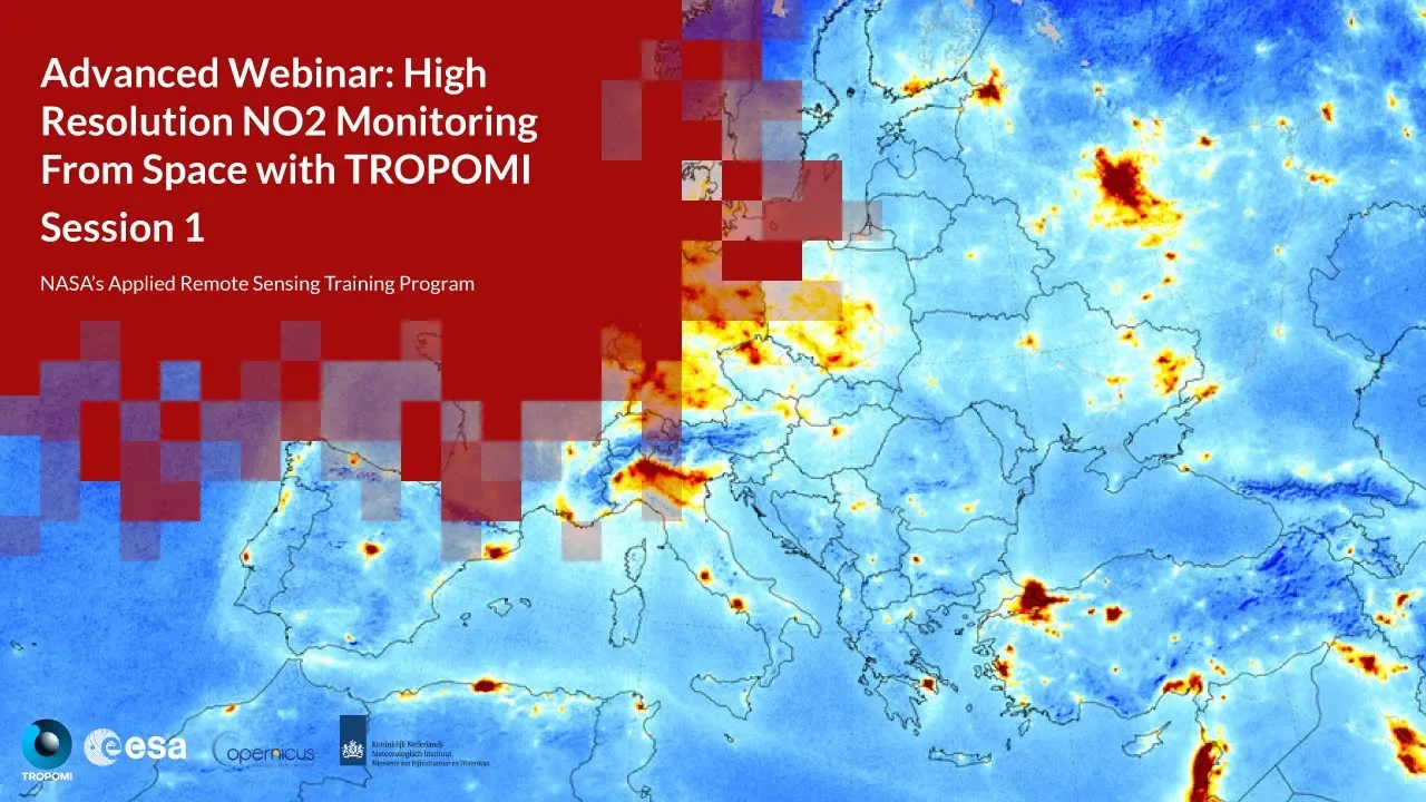
NASA ARSET: Remote Sensing of NO2 with OMI, Part 1/3
11.2K
Remote sensing collects information without physical contact using passive sensors dependent on solar radiation. Solar radiation passes through the atmosphere, interacts with surfaces, and returns with spectral signatures containing information about atmospheric constituents. Each trace gas has a distinct spectral fingerprint enabling identification. Passive sensors measure the entire atmospheric column, providing total column amounts but limited vertical information. Short-lived species like NO2 concentrate in the planetary boundary layer with large spatial gradients, while longer-lived species show weaker vertical variation. Data progresses through processing levels: Level 0 (raw), Level 1 (processed sensor units), Level 2 (geophysical variables), Level 2g (gridded without averaging), and Level 3 (gridded with averaging). Higher spatial resolution improves cloud clearing and reveals smaller sources. GOME-2 (2002) had 80x40 km² resolution; OMI improved to 24x13 km²; TROPOMI achieved 3.5x7 km². The OMI row anomaly affected 50% of data from 2007-2012. Future geostationary missions (TEMPO, Sentinel-4, GEMS) will provide hourly measurements over their regions.
Click to watch →
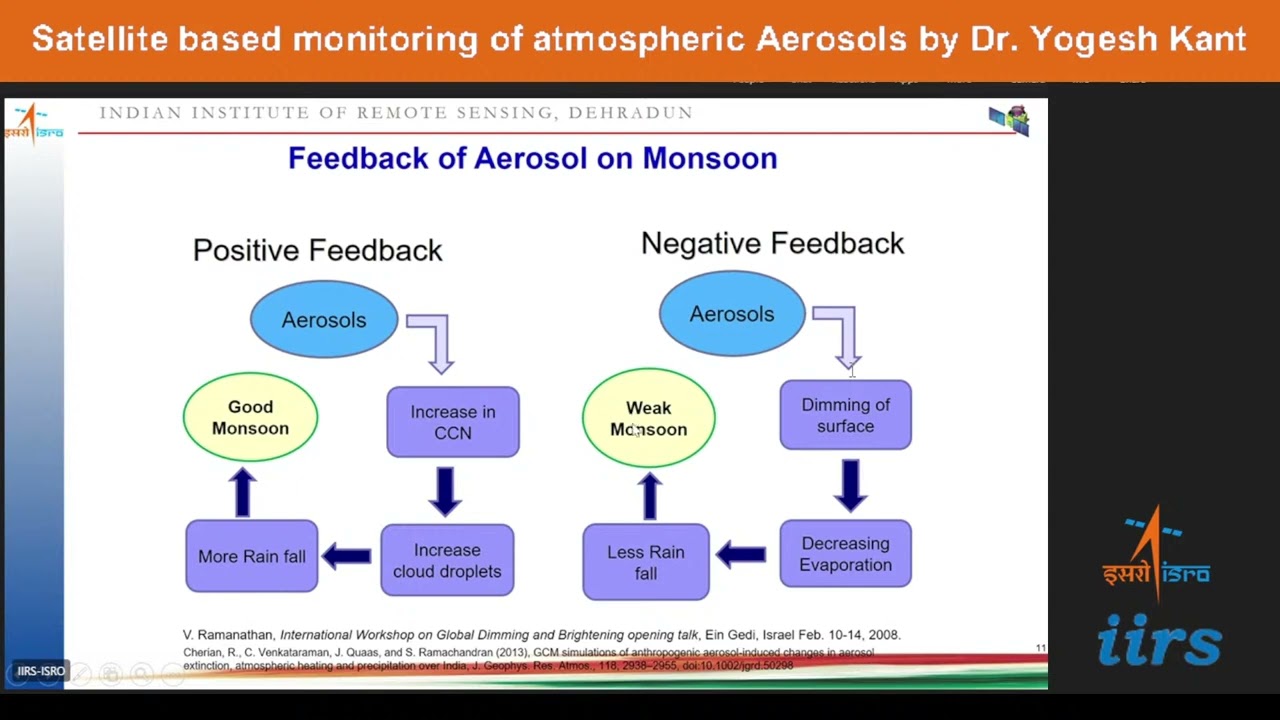
Satellite based monitoring of atmospheric Aerosols by Dr. Yogesh Kant
193
Aerosols are classified into three modes: Aitken mode (0.02-0.1 μm) from combustion, accumulation mode (0.1-1 μm) from coagulation, and coarse mode (>1 μm) from mechanical processes. Aerosol optical depth quantifies how much solar radiation is scattered or absorbed, determining what fraction reaches Earth's surface. Satellite remote sensing detects reflected solar radiation, measuring both reflected and emitted energy from atmospheric particulates. MODIS uses 36 spectral bands with Dark Target algorithms for ocean and land surfaces. MISR provides multi-angle observations (nine viewing angles) enabling aerosol loading estimation and particle size classification. TROPOMI offers 7x7 km resolution for simultaneous measurement of multiple atmospheric constituents including aerosols, ozone, and trace gases.
Click to watch →
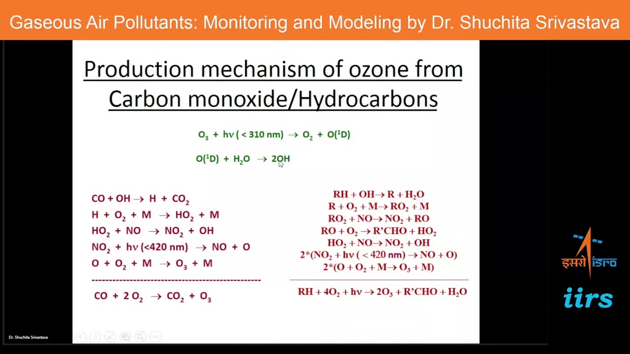
Gaseous Air Pollutants: Monitoring and Modeling Dr. Shuchita Srivastava
504
Satellite remote sensing detects backscattered solar or emitted terrestrial radiation to measure atmospheric composition. Each gas has a unique spectral fingerprint enabling identification. Differential absorption spectroscopy uses two closely spaced wavelengths—one strongly absorbed and one minimally absorbed—to calculate concentrations. OMI (2004) and TROPOMI (2017) are key instruments: OMI measures NO2, SO2, and O3; TROPOMI adds CO measurement with superior spatial resolution. These instruments enable global monitoring of pollution hotspots, long-range transport tracking, and detection of extreme events like volcanic eruptions and wildfires.
Click to watch →

Satellite based monitoring of gaseous air pollutants by Dr. Shuchita Srivastava
197
Satellite remote sensing detects atmospheric trace gases through absorption spectroscopy, exploiting unique spectral fingerprints of different gases in UV-visible and infrared ranges. Two main approaches exist: solar-reflected radiation (providing columnar information from surface to top of atmosphere) and emitted terrestrial radiation (revealing vertical distribution through Planck's law). Key instruments include OMI (Aura satellite, UV-visible, 2004+) and TROPOMI (Sentinel-5P, extended to near-infrared, 2017+), with progressively improving spatial resolutions enabling identification of pollution hotspots. These instruments enable global monitoring of pollutants like NO2, O3, SO2, and CO, providing data essential for understanding atmospheric chemistry and air quality on regional and global scales.
Click to watch →

Remote Sensing Application for Atmospheric Studies by Dr. Yogesh Kant
182
Remote sensing classifies into passive (using solar radiation) and active (emitting own signals) systems. Passive includes optical and microwave sensing; active includes lidar and radar. Electromagnetic radiation interacts with atmospheric constituents through scattering (larger particles) and absorption (molecules/gases at resonant frequencies). Atmospheric windows allow sensor detection. Different gases have unique absorption fingerprints (water vapor, ozone, CO, CH4, CO2, NOx, SO2) enabling identification and concentration estimation through Lambert-Beer law analysis.
Click to watch →
Deep Dive
The physics of meteoroid entry and airburst events, specifically how they vaporize and generate massive particulate plumes in the upper atmosphere.
What Would Happen If Asteroid Bennu Hit Earth?
394.5K
As asteroids enter Earth's atmosphere, dynamic pressure builds at their fronts, stripping material and causing fragmentation. Loosely bound rubble piles flatten into pancakes, increasing cross-section and accelerating deceleration—a feedback loop releasing massive energy. This airburst phenomenon, comparable to atomic explosions, occurs before ground impact. Atmospheric pressure at entry is ~10 tons/m², sufficient to disrupt even large objects. The Chelyabinsk meteor (20m, 13kt) exploded at 30km altitude, injuring 1,000 and damaging 2,000 buildings.
Click to watch →

Sumerische Aufzeichnungen enthüllen das FEUER, das Sodom und Gomorra auslöschte?
918
The asteroid approached Earth at a shallow 6-degree angle, skimming the atmosphere like a stone skipping across water. At 40,000 km/h, the air ahead compressed to temperatures exceeding 10,000°C—hotter than the Sun's surface. This compressed air, not direct friction, caused the asteroid's surface to melt and vaporize, creating a glowing plasma sheath. The object detonated in the atmosphere at 3-5 km altitude, releasing energy equivalent to over 1,000 Hiroshima atomic bombs. The horizontal shock wave then struck the ground, pulverizing the 15-meter-high city walls into microscopic dust.
Click to watch →
Impakte durch Meteoriten auf der Erde & im Sonnensystem • Planetare Geologie | Christian Köberl
227.8K
Many incoming meteoroids disintegrate in Earth's atmosphere before reaching the surface, producing airbursts that release enormous energy at altitude. The 1908 Tunguska event and the 2013 Chelyabinsk meteor demonstrate this phenomenon. Objects approximately 50 meters in diameter can explode in the atmosphere, generating shock waves capable of destroying forests over thousands of square kilometers. The Chelyabinsk event (2013) showed that objects about 20 meters in diameter can cause significant damage at ground level, with the explosion occurring at approximately 25 kilometers altitude. These events highlight that atmospheric entry physics significantly affects impact hazard assessment.
Click to watch →
![Прожарка научных мифов: самолеты, коллайдер, нанотехнологии, космический мусор. [СПЕЦВЫПУСК]](https://i.ytimg.com/vi_webp/-Uwyltzz8UE/maxresdefault.webp)
Прожарка научных мифов: самолеты, коллайдер, нанотехнологии, космический мусор. [СПЕЦВЫПУСК]
983.8K
The common belief that meteors burn up due to friction with atmospheric air is incorrect. When meteoroids enter Earth's atmosphere at speeds 30 times the speed of sound, they create shock waves that compress and heat the surrounding air to extreme temperatures (176 times normal). The meteoroid itself is surrounded by this superheated plasma, which causes it to vaporize. This process is called adiabatic heating - the rapid compression of gas molecules increases their velocity and thus temperature. The meteoroid is not being 'rubbed' by air but is surrounded by plasma generated by the shock wave ahead of it.
Click to watch →
Морозова Т.И. Загадочные явления в ионосфере Земли 06.03.2024 Трибуна молодого учёного
3.4K
During meteoroid passage, several processes occur: vaporization of meteoroid material, formation of a vapor cushion that slows the meteoroid, heating and melting of the surface, and formation of plasma tails. The vapor cushion forms from meteoroid atoms and slows the meteoroid. Molten material streams off the surface and solidifies into particles. Mechanical fragmentation can occur due to internal stresses. The plasma tail contains higher concentrations of electrons and ions than the surrounding ionosphere, with dust particle concentrations several orders of magnitude higher.
Click to watch →
Deep Dive
Fundamental concepts of atmospheric dynamics, including how global wind systems transport particles over time.

grade six unit three concept one lesson four
311
A global wind system is wind that blows in a fixed direction or for extended periods. Wind serves as a critical transport mechanism, moving rain, snow, clouds, and other atmospheric elements between locations. Two primary factors determine wind direction: solar radiation creates temperature differences between hot and cold regions, causing wind to flow from cold to hot areas; Earth's rotation deflects wind patterns from their original paths. These factors work together to create the global circulation patterns that distribute heat and moisture around the planet.
Click to watch →

SLST Geography IX-X & XI-XII | Series 26 | MCQ Practice | Planetary Wind System | নিয়ত বায়ু প্রবাহ
11.4K
This comprehensive section covers the fundamental principles of global wind systems and atmospheric circulation. Key topics include: (1) Wind classification into hot/dry, cold, mountain, and valley winds; (2) Permanent winds (Trade Winds, Westerlies, Polar Easterlies) versus non-permanent winds; (3) Coriolis force (discovered 1835) acting at right angles to wind direction; (4) Ferrel's Law and Buys Ballot's Law explaining wind deflection and pressure relationships; (5) Wind measurement instruments (Beaufort Scale, anemometer, wind vane); (6) Global circulation pattern from equator to poles: Doldrums, Trade Winds, Westerlies, Polar Easterlies; (7) Southern Hemisphere wind systems including Roaring Forties, Furious Fifties, and Screaming Sixties; (8) Local winds (Bora, Zonda, Khamsin, Foehn, Sirocco); (9) Three-Cell Circulation Model (Hadley, Ferrel, Polar Cells) with their associated wind systems and energy sources.
Click to watch →
वैश्विक पवन तंत्र: बस 1 वीडियो में पूरा टॉपिक खत्म! 😱 RPSC 2nd Grade GK Paper 1 | Short Notes
348
This comprehensive section covers the foundational principles of global wind patterns. Air pressure has inverse relationships with temperature, altitude, and humidity. The Earth has alternating pressure belts: Equatorial Low (0°), Subtropical High (30-35°), Subpolar Low (60-65°), and Polar High (90°). These belts are classified as thermal (formed by temperature differences) or dynamic (formed by air movement). The Coriolis force, caused by Earth's rotation, deflects winds and is zero at the equator but maximum at the poles. Trade winds blow from high to low pressure in the Hadley Cell: Northeast to Southwest in the Northern Hemisphere (5-30°N), Southeast to Northwest in the Southern Hemisphere (5-30°S).
Click to watch →

Geography for CDS 1 2023 | Study Funda
1.1K
Global wind systems are large-scale patterns of atmospheric circulation that transport heat and moisture around the Earth. The major systems include: (1) Trade Winds (0-30°) blowing from the subtropical high-pressure belts toward the equator (Northeast Trade Winds in the Northern Hemisphere, Southeast Trade Winds in the Southern Hemisphere); (2) Westerlies (30-60°) blowing from the subtropical highs toward the polar regions (Southwest Westerlies in the Northern Hemisphere, Northwest Westerlies in the Southern Hemisphere); (3) Polar Easterlies (60-90°) blowing from the polar high-pressure regions toward the mid-latitudes. These winds are deflected by the Coriolis effect due to Earth's rotation. The Hadley Cell is a major atmospheric circulation pattern that transports heat from the equator toward the poles, with warm air rising at the equator, moving poleward at high altitudes, and sinking at about 30° latitude.
Click to watch →

NIBRAS ONLINE CLASS | SSLC | GEOGRAPHY | CHAPTER 2 | IN SEARCH OF THE SOURCE OF WIND | PART 4
148
This comprehensive lesson covers the fundamental principles of global wind systems and atmospheric circulation. Wind is defined as the horizontal movement of air from high pressure to low pressure regions, influenced by pressure gradient force, Coriolis force, and friction. Winds are classified into planetary winds (large-scale consistent winds), periodic winds (seasonally changing), local winds (geographically influenced), and variable winds. The global wind system includes trade winds (blowing from subtropical high to equatorial low pressure: southeast trade winds in the southern hemisphere and northeast trade winds in the northern hemisphere, converging at the Intertropical Convergence Zone), westerlies (blowing from subtropical high to subpolar low pressure), and polar easterlies (blowing from polar high to subpolar low pressure). These wind systems form the backbone of global atmospheric circulation, driven by differential heating and the Coriolis effect.
Click to watch →
Prerequisite Knowledge
- Concept 01Understanding the thermal and physical structure of Earth's atmospheric layers, particularly the stratosphere and troposphere.
- Concept 02Basic principles of satellite remote sensing, including how sensors detect atmospheric aerosols and trace gases through spectral observations.
- Concept 03The physics of meteoroid entry and airburst events, specifically how they vaporize and generate massive particulate plumes in the upper atmosphere.
- Concept 04Fundamental concepts of atmospheric dynamics, including how global wind systems transport particles over time.
Subsequent Learning
- Step 01Advanced stratospheric transport mechanisms, such as the Brewer-Dobson circulation and polar vortex dynamics.
- Step 02Data assimilation techniques, which combine real-time satellite observations with computational atmospheric models to improve predictive accuracy.
- Step 03Analyzing the climatic impacts of high-altitude aerosol injection, drawing comparisons between volcanic eruptions and cosmic impacts.
- Step 04Exploring future atmospheric monitoring missions (such as JPSS and Sentinel-5P) and their enhanced capabilities for tracking aerosol events.
Meteor Explosion
Global Plume Spread
Meteor Explosion
0:00Playing Section
- 1
A massive meteor explodes above Chelyabinsk, Russia.
- 2
Satellite detects debris plume in the stratosphere.
- 3
NASA models accurately predict the plume's movement.
Resolution Limits of Satellite Tracking and Initial Plume Dynamics
While OMPS data on the Suomi NPP satellite offers broad global-scale tracking to validate stratospheric transport models, atmospheric scientists point out key limitations in this approach. Critics argue that satellite-based sensors lack the fine spatial and vertical resolution necessary to capture localized aerosol microphysics, such as particle coagulation and gravitational settling. Furthermore, standard global circulation models validated by OMPS often overlook the complex, high-altitude thermodynamics of the initial meteor explosion, including shockwave-driven dispersion and radiative self-lofting. Alternative perspectives suggest that ground-based lidar networks and high-resolution regional models reveal discrepancies in plume altitude and transport rates, indicating that relying primarily on low-resolution satellite data oversimplifies early-stage plume dynamics and stratospheric mixing.
Deep Dive
Advanced stratospheric transport mechanisms, such as the Brewer-Dobson circulation and polar vortex dynamics.

Imminent Polar Vortex Collapse over Antarctica will Impact Global Weather: My Deep Details Dive…
41.7K
The Brewer-Dobson circulation connects both hemispheres through atmospheric waves reaching 90 km altitude, enabling teleconnections where southern hemisphere disruptions influence northern hemisphere weather. Research shows 40-80% ionospheric electron content changes following stratospheric warming events, affecting radio transmission. Statistical correlations exist between southern August-October pressure anomalies and northern December-February temperatures, with prolonged southern high pressure predicting colder central/eastern US and warmer Europe. Recent peer-reviewed research reveals complex dynamics: stratospheric wave reflection over the North Pacific increases sudden stratospheric warming risks, leading to mid-latitude weather extremes. The polar vortex controls aerosol transport and ozone depletion over Antarctica. The 2022 Hunga Tonga eruption injected massive water vapor and sulfur dioxide into the stratosphere, reaching 58 km altitude and causing southern hemisphere cooling of 0.1°C without sustained polar vortex disruption.
Click to watch →

James Lee Dismantles the Chemtrail Narrative | Jerm Warfare
1.1K
This segment explores the atmospheric circulation patterns that determine how aircraft emissions affect the climate. The speaker explains that the Upper Troposphere Lower Stratosphere (UTLS) is a critical mixing zone at flight altitudes where aircraft emissions interact with atmospheric chemistry. The segment details how Brewer-Dobson circulation moves air from the troposphere into the stratosphere, where aircraft emissions accumulate rather than being washed out by rain. The speaker explains that once in the stratosphere, chemicals last much longer (3-5 months to a year) compared to the troposphere (2-4 weeks). The segment covers how the stratosphere is chemically different between hemispheres because 80% of all flights occur in the northern hemisphere. The speaker explains that Indian Space Organization measurements found 10,000 black carbon particles per cubic centimeter at 18 km altitude, which can only come from jet fuel being burned. The segment concludes that commercial aviation is effectively performing stratospheric aerosol injection on a massive scale without pumps and pipes.
Click to watch →

The Catastrophic Blizzards of Winter 1977-78: An Analysis
4.1M
The polar vortex is a counterclockwise circulation of the coldest air on Earth, strengthening in winter and weakening in summer. It doesn't exist as one unified circulation but shifts and can split into multiple smaller circulations. Sudden stratospheric warming occurs when air over thirty thousand feet above the North Pole warms tens of degrees Celsius over a few days, slowing or reversing the counterclockwise circulation. This is analogous to a spinning top that becomes unstable when it slows down. In 1977, even without major sudden stratospheric warming, October-December were well below average. When the event occurred in late December 1977, it was so strong that surface winds reversed direction north of 60 degrees latitude, allowing a blocking high to push the split polar vortex southward toward the Equator.
Click to watch →

The polar vortex - Crash Course #4
31.4K
The stratospheric polar vortex is a massive, spinning air current near Earth's poles that forms due to the temperature difference between the equator and poles, which creates strong pressure gradients and intensified winds through the thermal wind effect; this vortex acts as a barrier that keeps extremely cold polar air confined to high latitudes, but when it weakens or becomes displaced, it can allow frigid Arctic air to spill southward, dramatically affecting weather patterns at lower latitudes.
Click to watch →

Powerful X.5 Solar Flare.
22K
Sudden Stratospheric Warming (SSW) events cause rapid Arctic stratospheric temperature increases after extreme cold. During the week before Christmas 2023, temperatures dropped to -75°C, creating polar stratospheric clouds visible as far south as Italy. SSW events weaken the polar vortex, causing it to split or change direction. This allows cold Arctic air to spill down to lower latitudes. The 2018 UK cold wave was caused by such an event. When the jet stream shifts from east-west to north-south patterns, it pushes cold air southward, affecting weather patterns across North America.
Click to watch →
Deep Dive
Data assimilation techniques, which combine real-time satellite observations with computational atmospheric models to improve predictive accuracy.

Satellite data assimilation
260
Data assimilation combines numerical models with observational data to improve weather predictions. Numerical models are physics-based systems using conservation equations (mass, energy, momentum) solved through computer programming. Observations provide real-world measurements from satellites, ground stations, and ships. The process finds an optimal state that best matches both model and observations, improving initial conditions and future predictions. A cost function quantifies the difference between model and observations. The Ocean Surface Topography Mission (OSTM) launched by ISRO in November 2022 uses satellite altimeters to measure ocean surface height with 10-meter precision. Data assimilation systems combine multiple observation sources, assigning appropriate weights based on reliability and coverage to create comprehensive weather analysis.
Click to watch →
Grasping Publicly Available Aerosol Data Streams
110
Data assimilation is the mathematical process of combining observational data with model forecasts to produce improved initial conditions for weather prediction. At its core, it computes an error-weighted mean between observations (satellite, ground-based, aircraft) and model predictions. The process involves pre-processing data into standardized formats, applying quality control, characterizing observation errors including representativeness issues and spatial correlations, and using mathematical solvers to compute corrections. Innovation represents the difference between model background values and observations, while corrections adjust the model state accordingly. Ensemble approaches run models multiple times with slightly different initial conditions to quantify sensitivity and uncertainty. This iterative process creates prognostic error models that continuously improve forecast accuracy by incorporating real-time observational data into prediction systems.
Click to watch →

Satellite Data Assimilation in NWP Protect
980
Variational methods (3D-Var and 4D-Var) formulate data assimilation as an optimization problem, avoiding explicit matrix inversion by maximizing the joint probability distribution under Gaussian assumptions. This minimizes a cost function combining background and observation errors, solved iteratively using Newton-Raphson or conjugate gradient methods. 4D-Var extends this by incorporating observations at multiple time steps. The Kalman filter propagates background error covariance forward using the model itself, providing flow-dependent estimates but requiring prohibitive computational resources. The Ensemble Kalman Filter addresses this by using an ensemble of perturbed forecasts (typically 50-100 members) to approximate error statistics, providing flow-dependent error estimates while remaining computationally feasible. Hybrid methods combine variational optimization with ensemble-based error propagation. Satellite data contributes approximately 10% improvement in global numerical weather prediction skill, despite vast amounts of available data limited by assimilation constraints. Tropical cyclone track forecasting has improved 10-15% since the 1980s, though intensity prediction shows minimal improvement due to cloud-covered conditions blocking infrared observations. Approximately 80% of assimilated data comes from satellites while only 20% from terrestrial sources. Mass observations constitute ~70% while wind observations ~30%, with wind being particularly critical for tropical regions. Future improvements include assimilating cloud-effective observations, high-resolution geostationary satellites, space-based Doppler lidar, improved microwave assimilation, and enhanced vertical resolution during cloudy/rainy conditions.
Click to watch →

Цырульников М.Д. УСВОЕНИЕ ДАННЫХ МЕТЕОРОЛОГИЧЕСКИХ НАБЛЮДЕНИЙ: СОСТОЯНИЕ, ДОСТИЖЕНИЯ И ТЕНДЕНЦИИ
218
Data assimilation combines mathematical models of atmospheric systems with observations to estimate the true state. Modern atmospheric models reach billions of variables, requiring sophisticated approaches. Observations are classified into four categories: contact observations (radiosondes, surface stations), satellite observations (most numerous and valuable), remote sensing systems, and active radar systems. Satellite observations include temperature/humidity profilers, wind/cloud motion trackers, and radio occultation systems. Radar wind profiling measures wind through scattered signals. Microwave radiometers measure atmospheric temperature through brightness temperature. Infrared observations measure temperature through infrared emissions. Statistical analysis shows microwave observations contribute most to forecasting accuracy. Maximum likelihood interpolation is the most robust approach, with the Bayesian framework providing the mathematical foundation. Ensemble methods estimate the background error covariance matrix from multiple model realizations, avoiding computationally expensive full covariance calculations. Variational methods minimize cost functions balancing model and observation errors. The Ensemble Kalman Filter uses ensemble statistics to estimate background error covariance. Particle filters represent the posterior as discrete particles, useful for non-Gaussian distributions but prone to degeneracy. Four-dimensional variational methods assimilate observations over time windows with weak model constraints.
Click to watch →
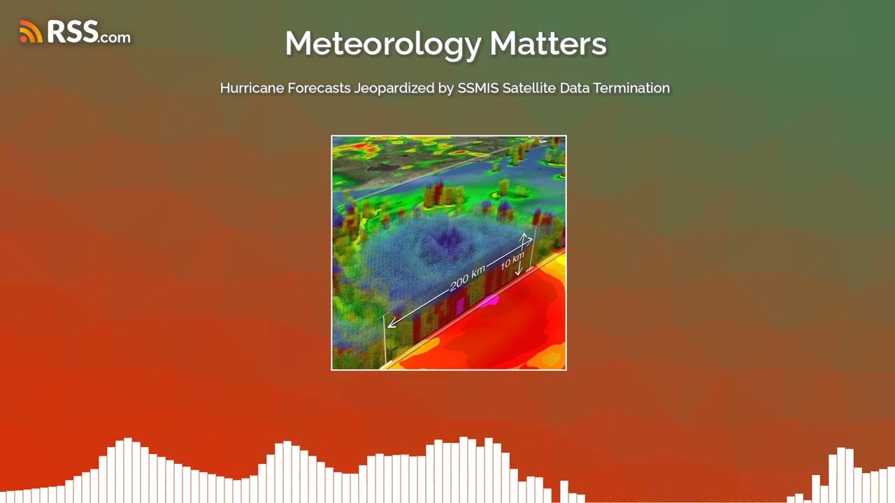
Hurricane Forecasts Jeopardized by SSMIS Satellite Data Termination
149
Weather prediction models rely absolutely on accurate initial conditions—precise data about the current atmospheric state, particularly moisture distribution. Conventional observations are too sparse over oceans to adequately sample fast-changing storm environments. Data assimilation techniques like 3D Variational systems integrate all available observations—including balloons, satellites, and other measurements—into the most consistent atmospheric picture. Two approaches exist for incorporating SSMIS data: assimilating retrieved products (statistical conversions) or directly assimilating raw brightness temperatures (physically-based methods). The raw TB method is more computationally intensive but more robust, better at reducing systematic biases. Hurricane Danny case studies demonstrate that assimilating SSMI data dramatically improves intensity and structure forecasts, reducing central pressure errors from 19.5 HPA to near-perfect predictions.
Click to watch →
Deep Dive
Analyzing the climatic impacts of high-altitude aerosol injection, drawing comparisons between volcanic eruptions and cosmic impacts.

Nano-Aerosole als Klimakühler? | #25 Nano Vorlesung Ganteför
11.4K
Major volcanic eruptions inject massive amounts of sulfate aerosols into the stratosphere (above 10 km altitude), which can significantly cool global temperatures. The 1815 Tambora eruption caused the 'Year Without a Summer' (1816), resulting in widespread crop failures, famine, and societal disruption across Europe and North America. Similarly, the 1991 Pinatubo eruption produced measurable but shorter-lived cooling effects. These historical events demonstrate that large-scale aerosol injection can override normal warming trends, providing evidence for aerosol-climate interactions that remain relevant to understanding current climate change discussions.
Click to watch →

Contact Report 594 Translation
127
Volcanic aerosols persist in the atmosphere for about 2 years after strong eruptions, interacting intensively with radiation by partially backscattering visible light and absorbing near-infrared and longwave spectrum radiation. This reduces solar radiation reaching Earth's surface while warming the stratosphere by approximately 25°C. These aerosols are chemically active, activating chlorine compounds that destroy the ozone layer. Whether small or large eruptions occur, they significantly contribute to atmospheric sulfur balance and are highly variable in space and time. Human-introduced sulfur aerosols in the lower troposphere also influence climate through radiative transfer. Volcanic aerosols in the stratosphere have effective radii matching visible sunlight wavelengths, making them particularly effective sunlight scatterers. Large eruptions reduce direct solar radiation while increasing diffuse radiation, causing skies to appear milky white during the day.
Click to watch →

COMO OS VULCÕES INFLUENCIAM O CLIMA?
1.2K
Volcanic eruptions affect climate only when they reach the stratosphere (12-15 km altitude). Eruptions below 5 km cannot affect climate because particles precipitate before reaching the stratosphere. When ash reaches the stratosphere, it undergoes chemical transformation: sulfur dioxide reacts with water to form sulfuric acid, creating sulfate aerosols with high reflectivity. These aerosols remain suspended for months to years, increasing planetary albedo and reflecting solar radiation back into space, causing global cooling. Historical evidence confirms this: Mount Pinatubo (1991) caused 0.5°C cooling; Krakatoa (1883) and Tambora (1815) caused similar effects; Laki (1783-1784) released 120 million cubic meters of sulfur dioxide, causing severe European cooling.
Click to watch →

Climats et sociétés humaines depuis deux mille ans (suite) (6) - Edouard Bard (2025-2026)
113
Major volcanic eruptions inject sulfur dioxide into the stratosphere, forming sulfate aerosols that increase Earth's albedo and cause cooling. Only eruptions sufficiently explosive to reach the stratosphere have climate impacts. The 43 BC Lockmok eruption in the Aleutians left traces in Greenland ice cores, demonstrating how volcanic activity can be identified through paleoclimate archives. These aerosols remain suspended for years, unlike tropospheric aerosols washed out by rain.
Click to watch →
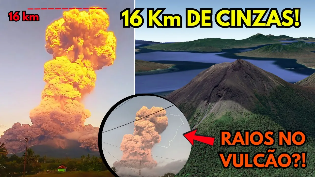
Explosão no Vulcão Lewotobi: Coluna de 16 km, Fluxo Piroclástico e Raio Vulcânico! Análise completa!
12.5K
When volcanic ash columns reach altitudes of 16 km or more, they enter the stratosphere, the second layer of Earth's atmosphere (above the troposphere, which extends to about 10-12 km). This high-altitude injection allows ash to disperse over larger regions, potentially affecting aviation and climate. Volcanic ash in the stratosphere can partially block solar energy, causing a temporary decrease in global average temperatures. The 1991 eruption of Mount Pinatubo demonstrated this effect, causing a measurable cooling of the Earth's climate for several years.
Click to watch →
Deep Dive
Exploring future atmospheric monitoring missions (such as JPSS and Sentinel-5P) and their enhanced capabilities for tracking aerosol events.

Aerosols and Climate Change - Philip Russell (SETI Talks)
1.8K
Future satellite missions aim to improve aerosol monitoring through advanced polarimetric and multi-sensor approaches. The Glory mission carries an Earth-viewing polarimeter designed to reduce reliance on models for aerosol property retrieval. The ACE (Aerosols, Clouds, and Ecosystems) decadal survey mission combines aerosol and ocean property observations on a single platform, featuring a multi-angle imaging spectropolarimeter, optical spectrometer, infrared scanner, lidar, and radar. This integrated approach addresses the challenge that aerosol and ocean retrievals are interdependent, requiring simultaneous optimization for both.
Click to watch →

Sentinel-5P prepared for liftoff
10.9K
Sentinel-5P, launched on 13 October 2017 from Plesetsk Cosmodrome on a Rockot launcher, is the first Copernicus mission dedicated to atmospheric monitoring. It carries the Tropomi instrument, which maps key trace gases including nitrogen dioxide, ozone, formaldehyde, sulphur dioxide, methane, carbon monoxide, and aerosols—substances critical to air quality, human health, and climate change. With a 2600 km swath width, it captures global atmospheric data daily. This information supports the Copernicus Atmosphere Monitoring Service for air quality forecasting, volcanic ash tracking for aviation safety, and UV radiation warnings to prevent skin damage. Scientists also use the data to enhance understanding of atmospheric processes, such as ozone layer depletion. Sentinel-5P was designed to bridge data gaps between the retired Envisat/Sciamachy mission and the upcoming Sentinel-5, while complementing GOME-2 on MetOp satellites. It is part of a future constellation including the geostationary Sentinel-4 and polar-orbiting Sentinel-5, both to be operated by Eumetsat for long-term atmospheric monitoring. The mission resulted from collaboration between ESA, the European Commission, the Netherlands Space Office, industry, and scientists, with Airbus Defence and Space UK and NL leading a 30-company consortium. Data from Sentinel-5P enables evidence-based environmental policy and public health decisions.
Click to watch →
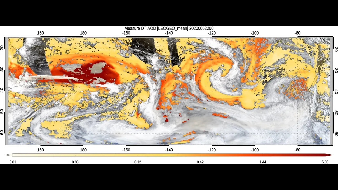
Introduction to NASA's GEO-LEO Dark Target Aerosol Data Products
680
NASA's GEO-LEO Dark Target Aerosol Data Products combine observations from geostationary (GEO) and low Earth orbit (LEO) satellites using a unified retrieval algorithm to monitor atmospheric aerosols with enhanced temporal resolution; the Dark Target algorithm identifies aerosols by detecting contrast between dark surfaces (oceans, vegetation) and airborne particles, producing Level 2 individual retrievals and Level 3 gridded products that increase observation frequency from once daily to every 10-15 minutes, enabling better tracking of rapidly moving aerosol plumes like those from wildfires and dust storms.
Click to watch →

EUMETSAT overview on aerosols. Webinar by Federico Fierli and Sabrina Szeto (EUMETSAT, Germany)
125
EUMETSAT, a European-based international organization with 35 contributing countries, provides comprehensive aerosol monitoring through multiple satellite platforms including geostationary Meteosat Second Generation and polar-orbiting satellites like Sentinel 3 and IASI, offering diverse aerosol products such as Aerosol Optical Depth, Absorbing Aerosol Index, and P-MAP synergistic products that combine data from multiple sensors to characterize dust properties, with future capabilities including Meteosat Third Generation and EPS-SG missions expected to enhance aerosol monitoring through improved polarization measurements and multi-spectral imaging.
Click to watch →

JPSS Satellites and the VIIRS Sensor
924
NOAA's JPSS (Joint Polar Satellite System) satellites, including Suomi NPP (launched 2011) and NOAA-20 (launched 2017), are polar-orbiting satellites at 824 km altitude that provide critical observations for weather prediction and environmental monitoring. The VIIRS (Visible Infrared Imaging Radiometer Suite) sensor on these satellites has 22 spectral bands with 750m resolution for M bands and 375m for I bands, offering a 3040 km swath width that provides full global coverage without tropical gaps, unlike heritage sensors like MODIS. The two satellites share the same orbit with observations approximately 50 minutes apart, enabling tracking of fast-evolving events like wildfires through multiple daily observations.
Click to watch →
Meteor Explosion
Global Plume Spread
Meteor Explosion
0:00- 1
A massive meteor explodes above Chelyabinsk, Russia.
- 2
Satellite detects debris plume in the stratosphere.
- 3
NASA models accurately predict the plume's movement.
Resolution Limits of Satellite Tracking and Initial Plume Dynamics
While OMPS data on the Suomi NPP satellite offers broad global-scale tracking to validate stratospheric transport models, atmospheric scientists point out key limitations in this approach. Critics argue that satellite-based sensors lack the fine spatial and vertical resolution necessary to capture localized aerosol microphysics, such as particle coagulation and gravitational settling. Furthermore, standard global circulation models validated by OMPS often overlook the complex, high-altitude thermodynamics of the initial meteor explosion, including shockwave-driven dispersion and radiative self-lofting. Alternative perspectives suggest that ground-based lidar networks and high-resolution regional models reveal discrepancies in plume altitude and transport rates, indicating that relying primarily on low-resolution satellite data oversimplifies early-stage plume dynamics and stratospheric mixing.
Understanding the thermal and physical structure of Earth's atmospheric layers, particularly the stratosphere and troposphere.
Basic principles of satellite remote sensing, including how sensors detect atmospheric aerosols and trace gases through spectral observations.
The physics of meteoroid entry and airburst events, specifically how they vaporize and generate massive particulate plumes in the upper atmosphere.
Fundamental concepts of atmospheric dynamics, including how global wind systems transport particles over time.
Advanced stratospheric transport mechanisms, such as the Brewer-Dobson circulation and polar vortex dynamics.
Data assimilation techniques, which combine real-time satellite observations with computational atmospheric models to improve predictive accuracy.
Analyzing the climatic impacts of high-altitude aerosol injection, drawing comparisons between volcanic eruptions and cosmic impacts.
Exploring future atmospheric monitoring missions (such as JPSS and Sentinel-5P) and their enhanced capabilities for tracking aerosol events.
574.1K views2.9Klikes3:50@NASAGoddardOriginal Release: 2013-08-14
(music) It's early morning on February 15th, 2013.
A meteor weighing 10,000 metric tons is about to explode nearly 23 km above Chelyabinsk.
Shortly after local sunrise: a blinding sight for the stunned spectators on the ground, (sound of explosion) a massive explosion equivalent to 440 kilotons of TNT, hundreds of tons of debris released, and quickly moved up into the atmosphere.
The highly sensitive OMPS instrument on board the Suomi/NPP satellite made its first observation of the plume nearly three and a half hours later, an entire 1,100km east of the explosion and already at 40km altitude well, into the Earth's stratosphere!
A surprising observation since the stratosphere usually acts as a bumper that caps aerosols trying to rise up from the lower atmosphere.
By inserting a column of data from the first plume observation into to two NASA models, scientists were able to project the plume's trajectory.
The models showed that the plume had higher altitudes, shown in red, would move ahead of the lower layer, shown in yellow.
The reason would be the difference in wind velocity at the lower and higher altitudes. Also illustrated here is how accurately the satellite observations coincided with the projected path of the plume.
(music) When OMPS made its second observation back at Chelyabinsk, nearly 5 hours after the bolide, there was still evidence of the plume at a lower 30km altitude.
On February 16, one day after the bolide, the OMPS instrument detected the far end of the plume even further, at 1,700 to 4,300 km eastward from the explosion.
By February 19th, four days after the explosion, the satellite observation showed that the meteor debris had circumnavigated the entire globe and returned to Chelyabinsk, forming a complete global belt.
The clean shape of the belt was another surprising prediction, considering that Northern hemisphere winds during the winter are usually rather inconsistent in direction.
A further look into the model simulation showed that evidence of the plume persist for a long time, which also coincided with the satellite observations.
We have now seen how accurately the models were able to project the plume's trajectory. This is critical since the same models are used to study climate and ozone depletion. The unprecedented sensitivity of the OMPS instrument and its ability to see vertical profile the atmosphere help scientists track and study the meteor plume for months, revealing a much better picture of what the aftermath on the atmosphere could be from potential future, and even bigger events.
(beeping)
Up Next

51:51
Asteroid Crater Geology & Astrophysics: Middlesboro, Kentucky (Impact Science)
@ScienceCircleFoundation
591 views•2023-02-25
61:17
First Billion Years of the Universe with the Square Kilometre Array
@iaaudc
121 views•2022-05-26
6:00
Asteroid Bennu: A Journey Through Solar System History | NASA
@NASAGoddard
752.3K views•2014-11-18

6:10
Gamma-Ray Bursts: Cosmic Snipers Explained | Astronomy
@kurzgesagt
15M views•2016-07-31
Related Study Plans & Knowledge Roadmaps
Structured learning paths in Astronomy
astronomy
Reionization: Pop III Stars, IGM & 21cm Line
01Foundations of Cosmology & the Early Universe
02Population III Stars & Cosmic Dawn
03Physical Mechanisms of Reionization
+ 2 more learning modules
17h5 modules
Explore Roadmap
astronomy
Planetary Rings: Dynamics, Roche & Resonances
01Foundations of Gravity and Orbital Mechanics
02Tidal Forces and the Roche Limit
03Structure, Composition, and Collisions
+ 2 more learning modules
10h5 modules
Explore Roadmap
astronomy
Asteroseismology: Stellar Waves, Ages & Cores
01Foundations of Stellar Astrophysics & Wave Mechanics
02Stellar Oscillation Modes: P-modes and G-modes
03Mathematical Framework of Asteroseismology
+ 2 more learning modules
35h5 modules
Explore Roadmap
astronomy
Adaptive Optics: Physics, Engineering & Control
01Foundations of Wave Optics and Wavefronts
02Atmospheric Turbulence & Optical Distortion
03Wavefront Sensing Technologies
+ 3 more learning modules
35h6 modules
Explore Roadmap