Python is a powerful, open-source programming language widely used in data science for tasks like modeling sales data, text mining, and building recommendation engines; this course teaches Python fundamentals including variables, lists, functions, and essential data science packages (NumPy, Matplotlib, Pandas) through interactive learning with instant feedback, requiring no prior technical knowledge.
Introduction to Python for Data Science | Microsoft & DataCamp Course
Added:Deep Dive
Basic computer literacy, including file management and familiarity with using an Integrated Development Environment (IDE) or Jupyter Notebooks.

COMO UTILIZAR O JUPYTER NOTEBOOK?
55.6K
Jupyter Notebook is an integrated development environment for developing code in workshops and courses. It combines text and code in a single interface, facilitating explanation and understanding of code execution steps. Anaconda installation includes Jupyter Notebook, making it accessible for beginners. The platform allows real-time code execution and result observation. Three launch methods exist: Anaconda Navigator, command line (jupyter notebook), and system search. File management includes creating new files, uploading files from computer, and opening existing notebooks through the file explorer interface.
Click to watch →

Python for data analyst | day 01 | 30 days free course | beginners to advance | python with project
945K
An Integrated Development Environment (IDE) combines multiple development tools into a single graphical interface, providing facilities for writing code, running programs, and debugging errors. Before IDEs, developers had to write code in one place, run it in another, and compile it in a third, which was time-consuming. Popular Python IDEs include PyCharm, VS Code, Sublime Text, and Jupyter Notebook. Jupyter Notebook is an interactive environment for creating and sharing computational documents, allowing users to write code, run it, and visualize results all in one place. It supports multiple programming languages but is most commonly used with Python, enabling users to write code cells, execute them, and immediately see the output. It is used by approximately 57% of data professionals.
Click to watch →

لو سمحت من غير كحول #عديل_الروح
79.2K
Basic computer literacy involves understanding how to transfer files between devices, use storage media like CDs and USB drives, and navigate software programs. These fundamental skills enable individuals to manage digital content efficiently and troubleshoot common technical issues.
Click to watch →

GSRTC CONDUCTOR 2026 | ટિકિટ | કમ્પ્યૂટરમાં પૂરા માર્ક્સ પાક્કા | LIVE 5:00 PM | HIREN Sir
6.1K
This section covers computer literacy concepts and file management. Computer Literacy Day is celebrated on December 2nd. India's first search engine is called 'Khoye'. A file extension indicates the file type and format, such as .txt for Notepad files. The Tab key moves the cursor by five spaces, and Ctrl+D duplicates slides in presentation software.
Click to watch →
Aula 1 - Fundamentos da programação - Programação Estruturada 2025
414
Jupyter Notebook is an integrated development environment that uses the browser to display files and folders. It shows the computer's file system with a different interface. Users can create new folders and files directly within Jupyter, and these appear in the actual computer file system.
Click to watch →
Deep Dive
Fundamental mathematical concepts, specifically basic algebra (variables, coordinate grids) and elementary statistics (mean, median).

رياضيات الاول متوسط 2025 | الفصل الثالث | الحد الجبري والحدود المتشابهة |محاضرة1 |
307.8K
This lesson introduces three foundational algebraic concepts. A variable is any letter from the English alphabet (x, y, z, w, a, b, i) that represents an unknown value. The coefficient is the numerical value that multiplies the variable (e.g., in 5y, the coefficient is 5). An algebraic term combines a coefficient with a variable (e.g., 2x, 4z, 5y). These concepts form the building blocks for understanding more complex algebraic expressions and equations.
Click to watch →

حل تمارين رياضيات (جبر) الصف الثاني الاعدادي ـ علي الفصل الدراسي الاول، مراجعة امتحانات يناير ج2
176
This comprehensive lesson covers two major mathematical topics. First, coordinate geometry: three points are collinear if slopes between any two pairs are equal, calculated as (y2-y1)/(x2-x1). Horizontal lines have slope 0, vertical lines have undefined slope. Second, statistics: the arithmetic mean is sum of values divided by count. In frequency distributions, class marks are midpoints calculated as (lower+upper)/2. The mean from frequency tables is Σfx/Σf. These concepts form foundational skills for algebra and data analysis.
Click to watch →

" مراجعة ليلة الإمتحان " رياضيات " للصف السادس الإبتدائي | مستر محمد جمعه
216
This section covers algebraic and statistical concepts: (1) Algebraic expressions - combinations of numbers, variables, and operations; (2) Simplifying expressions by combining like terms; (3) Solving equations with variables on both sides; (4) Independent and dependent variables - independent variables change or are controlled, dependent variables respond to changes; (5) Descriptive statistics: mode (most frequent), median (middle value), mean (average), range (max minus min); (6) Choosing appropriate measures - median preferred when data has outliers; (7) Order of operations (PEMDAS): Parentheses, Exponents, Multiplication/Division, Addition/Subtraction.
Click to watch →

College Algebra Topic 1.2 Video
4.3K
This comprehensive section covers two major topics in college algebra. First, one variable data analysis includes calculating maximum, minimum, mean (average), median (middle value), mode (most frequent), and range (max minus min). The calculator STAT function provides these statistics automatically. Second, coordinate geometry covers the distance formula D = √[(x₂ - x₁)² + (y₂ - y₁)²) for finding distances between points, and the midpoint formula (x₁ + x₂)/2, (y₁ + y₂)/2) for finding center points. These formulas are applied to coordinate plane problems and real-world estimation scenarios.
Click to watch →

Class 10 | Math Objective | Internet Model paper 2022 | set -3 | Part 1 by nagendra 🔥🔥🔥🔥🔥
4.1K
This segment covers essential statistical concepts and coordinate geometry fundamentals. The mean (average) is calculated by summing all values and dividing by the count. The mode is the most frequently occurring value. The median is the middle value when data is ordered. In coordinate geometry, points are represented as ordered pairs (x, y), with the origin at (0,0). Points on axes have coordinates (x,0) or (0,y). The class mark (midpoint) of an interval is found by averaging the lower and upper limits. These foundational concepts are essential for understanding data analysis and geometric representations.
Click to watch →
Deep Dive
A conceptual understanding of how data is structured and stored, such as in spreadsheets, tables, rows, and columns.
Introduction to SQL in Salesforce Marketing Cloud: Lesson 1 - Introduction
19.8K
A table is a structured database object that contains data, organized using rows and columns similar to an Excel spreadsheet. Columns are also referred to as fields, and rows are also referred to as records. The values stored within these fields and records are called data. This structured format allows for easy retrieval of specific data by providing an address to look up.
Click to watch →

Components of Data Explained
1.6K
A spreadsheet is a tool for organizing data in a tabular format. Tables can be created on paper or digitally. Digital spreadsheets like Microsoft Excel and Google Spreadsheets offer unlimited rows and columns. Columns run vertically (top to bottom) and are labeled with letters (A, B, C, D). Rows run horizontally (left to right) and are labeled with numbers (1, 2, 3, 4). The intersection of a column and row creates a cell, which is the smallest unit in a spreadsheet. Each cell has a unique address formed by combining the column letter and row number (e.g., A1). A workbook is the digital equivalent of a notebook containing multiple sheets for organizing different types of data.
Click to watch →
Introduction to Database ସମ୍ପୂର୍ଣ୍ଣ ଓଡ଼ିଆରେ | +2 2nd Year CHSE | Database Fundamentals L-1
930
A table is a collection of related data in an organized manner, represented as a two-dimensional structure of rows and columns. A table is a 2D representation of a relation consisting of rows (also called records or tuples) and columns (also called fields or attributes). A row is a horizontal representation containing specific information for each entry in the table. A column is a vertical entity containing all information associated with a specific field. For example, in a student table, the 'agent name' column contains all information about agent names, while each row represents a single student's complete information.
Click to watch →

1-5 Conceptos básicos de una Planilla de Cálculo
1.2K
Spreadsheets are organized into columns (vertical spaces) and rows (horizontal spaces). Columns are identified by letters (A, B, C, etc.) and rows are identified by numbers (1, 2, 3, etc.). The intersection of a column and row creates a single cell.
Click to watch →
Como aprender SQL rápido | Em 8 minutos
547
A database can be conceptualized as a giant interconnected spreadsheet file. Instead of spreadsheets, databases use tables. Tables consist of rows (containing stored information) and columns (representing fields or attributes). Tables can represent specific types of information such as customer records, sales data, or inventory management.
Click to watch →
Deep Dive
Logical reasoning and algorithmic thinking, which are essential for understanding how code executes step-by-step.

Como estudar lógica de programação sozinho | ajudando iniciantes - parte um
12.9K
Programming logic is the organization of clear instructions for solving problems or creating software. An algorithm is the narrative of these instructions. Everyday activities like morning routines represent algorithms—sequences of actions where each step leads to the next. Programming involves sequencing things in stages, which is essential because computers cannot predict actions like humans can. The more detailed an algorithm is, the more efficient and bug-free it becomes. Programming logic must be studied before any programming language because while languages have different syntax and data types, the underlying logic remains the same. Programming is fundamentally about solving problems for companies or clients. To develop logical thinking, one should break down tasks into smaller steps and create the habit of thinking about how things work. Everything done in sequence of actions is an algorithm. Creating the habit of thinking analytically about routine actions stimulates logical thinking.
Click to watch →

92.1 - NOÇÕES BÁSICAS DE MATEMÁTICA COMPUTACIONAL - MATEMÁTICA - 1º ANO E.M - AULA 92.1/2023
801
Logical reasoning is the method of organizing thoughts and demonstrating reasoning correctly. It involves using premises to reach conclusions. An algorithm is a sequence of logical steps that leads to a specific objective. Practical examples include Bhaskara's formula for solving quadratic equations and step-by-step procedures like changing a light bulb. Algorithms can be represented by equations or described paths, providing systematic approaches to solving problems.
Click to watch →

Lecture 4 - Introduction to Coding - What is an algorithm? | Coding For Juniors Complete Course
109
Algorithms are practical step-by-step plans for completing tasks. Making a sandwich demonstrates algorithmic thinking: take bread, open jam, spread jam, place second bread, eat. Each step must follow logically from the previous one. Logic in algorithms means understanding why each step is performed—bread must be taken first because it forms the base. If any step is forgotten or performed in the wrong order, it creates a bug. Debugging fixes these errors. A cooking recipe is essentially an algorithm, providing a sequence of steps to achieve a desired outcome.
Click to watch →
![[CS]컴퓨팅 사고력 - 알고리즘적으로 생각하기](https://i.ytimg.com/vi/PYB32Qx-etk/maxresdefault.jpg)
[CS]컴퓨팅 사고력 - 알고리즘적으로 생각하기
5K
This module introduces algorithmic thinking as an advanced step in logical and computational reasoning. An algorithm is defined as a process or set of rules to be followed in calculations or problem-solving operations. Examples include cooking recipes, science lab procedures, Lego instruction sets, and airplane emergency manuals. Computer programs are algorithms containing step-by-step instructions. Pseudo code allows expressing algorithmic ideas in a language-independent manner, enabling abstraction and sharing of concepts. Mathematical formulas like the distance formula and Pythagorean theorem serve as algorithms. Functions and blocks enable code abstraction and reuse, making programs cleaner and more elegant.
Click to watch →

Lógica de programação, por onde começar ? (Guia RÁPIDO de estudos completo para INICIANTES)
809.8K
An algorithm is defined as a sequence of steps or instructions designed to solve a specific problem or accomplish a particular task. To illustrate this concept, consider assembling a piece of furniture like a gaming chair: the manufacturer provides a manual containing all the necessary steps—connecting pieces together using specific screws in a particular order—to successfully complete the assembly. Similarly, when baking a cake, there exists a logical sequence of actions: gathering ingredients first, mixing them properly, preheating the oven before placing the mixture inside. The critical insight is that algorithms require proper sequencing; if steps are disorganized or out of order, the intended outcome cannot be achieved. This everyday reasoning forms the basis of algorithmic thinking in programming.
Click to watch →
Prerequisite Knowledge
- Concept 01Basic computer literacy, including file management and familiarity with using an Integrated Development Environment (IDE) or Jupyter Notebooks.
- Concept 02Fundamental mathematical concepts, specifically basic algebra (variables, coordinate grids) and elementary statistics (mean, median).
- Concept 03A conceptual understanding of how data is structured and stored, such as in spreadsheets, tables, rows, and columns.
- Concept 04Logical reasoning and algorithmic thinking, which are essential for understanding how code executes step-by-step.
Subsequent Learning
- Step 01Advanced data manipulation and cleaning techniques using pandas (such as merging datasets, grouping data, and handling missing values).
- Step 02Exploratory Data Analysis (EDA) workflows and statistical data visualization using advanced libraries like Seaborn or Plotly.
- Step 03Fundamental Machine Learning algorithms and model building using the Scikit-Learn library.
- Step 04SQL and relational database management for retrieving and querying data before processing it in Python.
Course Intro
Course Intro
0:00Playing Section
- 1
Introduces Python for data science course.
- 2
Covers basics, packages, and interactive learning.
R as the Superior Alternative for Statistical Data Science
While Python is a dominant general-purpose language for machine learning, many statisticians and researchers argue that R is a superior language for learning and practicing data science. Developed specifically for statistical computing and graphics, R offers a highly intuitive environment for data exploration, manipulation, and visualization through its 'tidyverse' ecosystem and 'ggplot2' package. Critics of a Python-first approach argue that Python's syntax can be overly verbose and geared toward software engineering, whereas R allows beginners to perform complex statistical modeling and generate publication-quality visualizations with fewer lines of code. For students focusing primarily on data analysis, statistical inference, and business intelligence—rather than software deployment—starting with R provides a more specialized and intellectually direct pathway.
Deep Dive
Advanced data manipulation and cleaning techniques using pandas (such as merging datasets, grouping data, and handling missing values).

#1 - Data Cleaning in Pandas Python(Advanced)
6.5K
This tutorial covers advanced Pandas data cleaning techniques including data type conversions using astype() and to_numeric(), date format handling with to_datetime(), string manipulation methods like str.lower() and str.contains(), DataFrame operations such as concat(), merge(), transpose(), melt(), pivot(), and stack/unstack, and data imputation using fillna() with median values to handle missing data.
Click to watch →

Day 2 | Data Manipulation and Analysis
1.9K
To merge two data frames, use pd.merge(left, right, on='key') to combine data from multiple tables based on a common key column. df.groupby('column') groups data by column values, allowing aggregation functions like sum or mean to be applied to each group. Grouping by multiple columns creates a multi-index (hierarchical index). df.stack() converts a data frame with multi-index into a series, and df.unstack() is the inverse operation. Time series data changes over time, and Pandas provides specialized functions for handling it. Pandas can also handle categorical data. To import data, use pd.read_csv() or pd.read_excel(). Data cleaning is crucial, involving diagnosing problems using head(), describe(), and visualization. Common problems include missing values, incorrect data types, coordinate columns containing strings, currency symbols, and out-of-range values. To split coordinate columns, use df['column'] = df['column'].str.split(','). To remove currency symbols, use df['column'] = df['column'].str.strip('$'). Convert to float using df['column'] = df['column'].astype(float). To replace categorical values, use df.replace({'old': 'new'}). To drop irrelevant columns, use df.drop(columns=['column']). To remove duplicate records, use df.drop_duplicates().
Click to watch →

Pandas Introduction ULTIMATE Guide: What Is Pandas, Why DataFrames Are Essential & Installation
457
Pandas provides comprehensive tools for data manipulation and cleaning. Key operations include: (1) Data filtering and conditional changes - filtering data by simple and compound conditions, (2) Data filtering and updations - retrieving and updating data using conditions, (3) Working with duplicate values - knowing about duplicates and removing them, (4) Working with missing data - understanding missing values (None, np.nan, pd.NA), finding, filling, and removing missing values, (5) Renaming DataFrame columns, (6) Merging DataFrames, (7) Data set reshaping - changing structure (columns to rows or vice versa), (8) Importing and exporting data - loading data from files (primarily CSV files, used 90-99% of the time) and saving processed data back to files, (9) Adding new columns to existing DataFrames, (10) Removing columns from DataFrames, (11) Adding new rows to DataFrames, and (12) Removing rows from DataFrames. Group By transformations are advanced operations for data analysis involving: (1) Loading data, (2) Grouping data based on specific criteria (e.g., grouping electoral data by state), (3) Transforming grouped data (applying functions to each group), and (4) Filtering results. This enables statistical analysis and aggregation of data across different categories.
Click to watch →
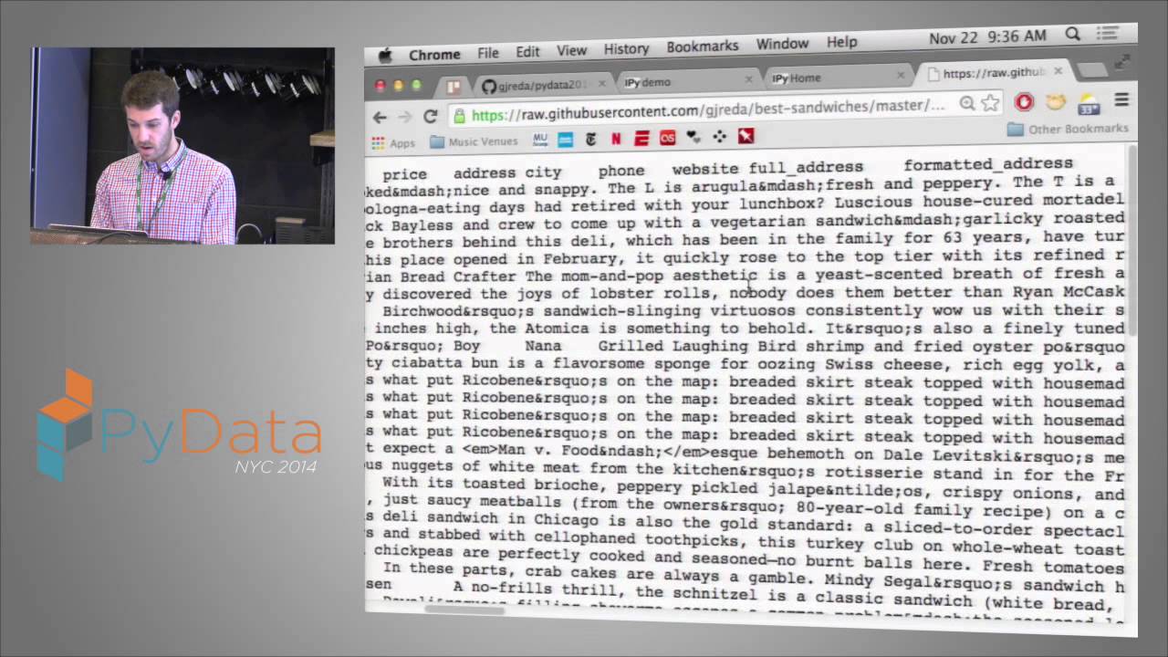
Greg Reda - Translating SQL to pandas. And back.
28.9K
Advanced data manipulation in Pandas involves combining datasets and applying operations efficiently. The merge() function performs SQL-style joins (left, right, inner, outer) between DataFrames using specified columns, with customizable suffixes for conflicting column names. The concat() function combines multiple DataFrames vertically, stacking them with NaN values for mismatched columns. The split-apply-combine methodology underlies most analytical workflows: groupby() splits data into groups, then apply aggregation functions like size(), mean(), and median(). The agg() method allows applying multiple functions to different columns simultaneously. These techniques enable efficient handling of large datasets and complex data transformations typical in real-world analysis workflows.
Click to watch →
“Complete Pandas Tutorial for Data Science | Hands-on Coding Session”
410
Data manipulation includes adding columns with 'df[new_col] = values' or calculations, dropping columns with 'df.drop(columns=[cols], axis=1)', and renaming columns with 'df.rename(columns={old:new})'. Value replacement uses 'df[column].replace(old, new)'. Grouping uses 'df.groupby(column)' for single-level and 'df.groupby([cols])' for multi-level grouping. Aggregation functions include 'count()', 'sum()', 'mean()', and 'std()'. Sorting uses 'df.sort_values(by=col, ascending=True/False)' for single columns and 'df.sort_values(by=[cols], ascending=[bools])' for multi-level sorting. Missing value handling uses 'fillna(value, inplace=True)' to replace nulls and 'dropna(inplace=True)' to remove rows with nulls. Data merging uses 'concat()' for stacking, 'join()' for key-based merging, and 'merge()' for SQL-like joins. Pivot tables summarize data using 'pd.pivot_table(df, values=col, index=rows, columns=cols, aggfunc=func)'. Function application uses 'df.apply(function, axis=0/1)' for row-wise or column-wise operations.
Click to watch →
Deep Dive
Exploratory Data Analysis (EDA) workflows and statistical data visualization using advanced libraries like Seaborn or Plotly.
Comprehensive Guide on MATPLOTLIB, SEABORN & PLOTLY | Python Data Analysis
9.5K
This video tutorial provides a comprehensive guide to three essential Python visualization libraries: Matplotlib for foundational static plots (histograms, bar charts, line charts), Seaborn for aesthetically pleasing statistical visualizations with minimal code, and Plotly for interactive web-based dashboards and real-time data exploration. The instructor demonstrates practical examples using Apple stock data, including techniques for creating histograms, bar plots, line charts, 3D scatter plots, and heatmaps with each library, while explaining key parameters like bins, colors, transparency, labels, and legends. The tutorial emphasizes choosing the right tool based on project requirements—Matplotlib for basic static visualizations, Seaborn for quick statistical insights, and Plotly for dynamic interactive visualizations—and shows how these libraries can be combined for maximum productivity in data analysis workflows.
Click to watch →
15 Python Libraries You Should Know About
454.5K
Seaborn is a Python library built on top of Matplotlib for creating statistical data visualizations. It simplifies the process of generating beautiful charts and graphs by providing default styles and themes that produce publication-quality visualizations with minimal configuration. Users provide data and basic settings, and Seaborn handles the rest. The library includes various themes (dark, white, ticks) and color palettes that allow visualizations to match the aesthetic of applications. This makes it ideal for exploratory data analysis where quick, attractive visualizations are needed without extensive customization.
Click to watch →
Sesión 5 Análisis de Datos
8K
Seaborn is a higher-level library built on Matplotlib that simplifies creating complex plots with less code, providing pre-styled themes and easier access to common plot types. Violin plots show data distribution using box plots combined with kernel density estimates, with hue parameter for categorization. Crosstab() creates frequency tables from two columns. DataFrames can be filtered using boolean indexing or loc/iloc methods. Normalization divides values by row/column sums to convert to percentages. Stacked bar charts use barplot() with stacked=True and hue parameter for additional categorization. Confidence intervals show the range within which the true population parameter likely falls, with default 95% confidence. Themes and palettes can be customized using set_theme() and set_palette().
Click to watch →
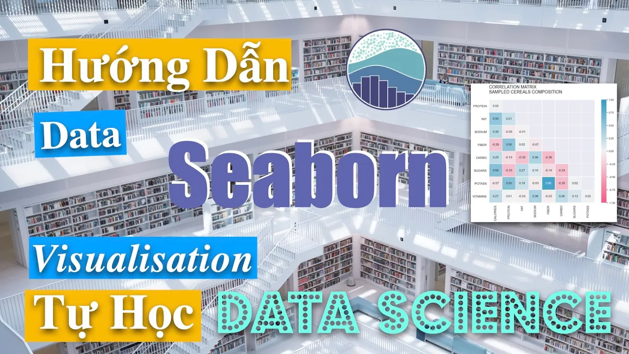
Hướng Dẫn Trực Quan Hoá Dữ Liệu với Seaborn và Python
43.7K
Seaborn is a Python data visualization library built on Matplotlib that provides high-level interfaces for creating statistical graphics, enabling users to easily visualize data distributions, relationships, and patterns through various plot types including histograms, KDE plots, bar plots, box plots, facet grids, joint plots, and heatmaps, making complex data analysis more accessible and visually informative.
Click to watch →

3.4. Seaborn Tutorial in Python | Machine Learning Course
48.3K
Seaborn is a Python data visualization library built on top of Matplotlib that simplifies the creation of complex statistical plots; it provides high-level interfaces for generating various types of plots including scatter plots, count plots, bar charts, distribution plots, and correlation heatmaps, with features like automatic styling, faceting, and theming that make it more efficient than using Matplotlib directly for exploratory data analysis in machine learning workflows.
Click to watch →
Deep Dive
Fundamental Machine Learning algorithms and model building using the Scikit-Learn library.
Real-World Python Machine Learning Tutorial w/ Scikit Learn (sklearn basics, NLP, classifiers, etc)
262.4K
Machine learning follows a systematic pipeline: define the problem, gather data, preprocess, build models, evaluate, and fine-tune. Scikit-learn simplifies this by providing pre-packaged implementations of common algorithms. The library primarily supports traditional algorithmic models (SVM, decision trees, naive Bayes, logistic regression) rather than deep learning approaches. Understanding both theoretical foundations and practical implementation is essential for effective model development.
Click to watch →

Jake VanderPlas: Machine Learning with Scikit Learn
45.8K
Machine learning builds models with tunable parameters that adapt to training data for generalization. Classification distinguishes discrete categories by finding separating boundaries, while regression predicts continuous values. Both scale to high dimensions where manual separation is impossible. scikit-learn requires data in two-dimensional matrices where rows are samples and columns are features, with labels stored separately. The Iris dataset demonstrates this structure: 150 flower samples with 4 measurement features and 3 class labels. Feature engineering—the process of selecting relevant numerical features—is critical and requires domain expertise. PCA helps select important features from larger candidate sets. scikit-learn implements a consistent estimator API where models are classes instantiated with hyperparameters, fitted to data, and used to make predictions. Supervised learning uses labeled data to train predictors. K-Nearest Neighbors classifies by finding nearest neighbors and taking majority votes. Support Vector Machines find optimal hyperplanes by maximizing margins between class clusters, focusing only on support vectors near boundaries. This makes SVMs robust to outliers. Linear regression fits linear functions to predict continuous targets by minimizing residuals.
Click to watch →
PYTHON SKLEARN: KNN, LinearRegression et SUPERVISED LEARNING (20/30)
336.9K
Machine learning enables machines to learn without explicit programming by developing mathematical models from data. The three main techniques are supervised learning (predicting Y from X), unsupervised learning, and reinforcement learning. In supervised learning, features (X) and targets (Y) are used to train models for regression (continuous Y) or classification (discrete Y). Scikit-learn implements all models using an object-oriented architecture where each model is an 'estimator' with fit(), score(), and predict() methods. Data must be two-dimensional with samples as the first dimension. Linear regression works for linear data but fails for non-linear data, requiring alternative models like SVM or feature engineering.
Click to watch →
Learn Machine Learning Like a GENIUS and Not Waste Time
1.1M
Scikit-learn is the number one machine learning library in the world for basic machine learning algorithms. A basic scikit-learn tutorial can be completed in one or two days. Its simple and consistent syntax means once you know how to use it for one algorithm, you know how to use it for any algorithm, provided you understand what each algorithm is meant for. The library comes with great documentation and toy datasets for practice. It is recommended to start using scikit-learn while learning about algorithms in the statistical learning course, implementing algorithms in three ways: from scratch using basic Python, using scikit-learn, and applying both approaches to real datasets.
Click to watch →
Como Treinar Modelos de Machine Learning com Sklearn
3.1K
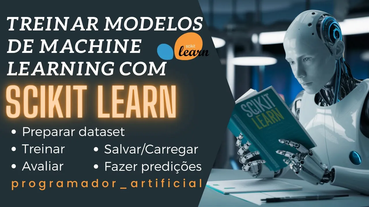
This comprehensive section covers the foundational workflow of machine learning using scikit-learn. Key topics include: (1) Understanding scikit-learn as a foundational library used by major companies, (2) Data preparation including handling missing values through mean imputation or row removal, (3) Train-test splitting (70/30) to prevent data leakage, (4) Data scaling using StandardScaler trained only on training data, (5) Model training with Decision Trees and configurable parameters, (6) Evaluation using accuracy and confusion matrices, (7) Feature importance analysis to identify relevant predictors, (8) Tree visualization for interpretability, and (9) The trade-off between model complexity and training time. The video emphasizes that proper preprocessing and understanding of model mechanics are essential for successful machine learning projects.
Click to watch →
Deep Dive
SQL and relational database management for retrieving and querying data before processing it in Python.
Python DatabaseProgrammingPart2
167
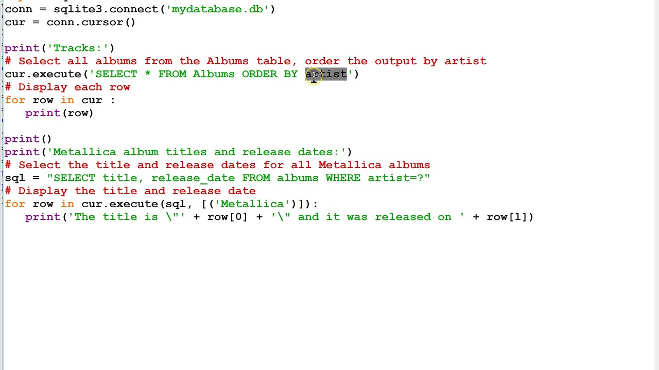
After creating database tables, the primary purpose is retrieving information through queries. The SELECT statement retrieves data with syntax: SELECT columns FROM table WHERE condition ORDER BY column. The asterisk (*) retrieves all columns, while specific columns can be listed separated by commas. The WHERE clause filters records using conditions, and parameter substitution (question marks) prevents SQL injection while allowing dynamic values. The cursor.execute() method runs queries, and cursor.fetchall() returns results as a list of rows. Each row is accessed by column index (row[0], row[1], etc.). Python can connect to various databases including SQLite, Oracle, MySQL, and PostgreSQL.
Click to watch →

B3 Le Langage SQL #5
1.9K
SQL is a powerful database management language, while Python is a powerful programming language. Their combination creates an ideal pairing for applications. The workflow involves: importing sqlite3, connecting to the database (creating it if needed), creating a cursor for manipulation, executing SQL queries, and processing results. Key methods include execute() for running queries, fetchone() for single rows, and fetchall() for all rows. Data is returned as lists of tuples. Essential practices include committing changes with commit() and closing both cursor and connection before ending the program.
Click to watch →

Python y la gestión de bases de datos
487
A database is a collection of data stored in the same physical support for subsequent use, with most modern databases being relational (data organized in related tables). SQL (Structured Query Language) is the standard programming language for accessing relational databases, enabling operations like calculations and relational algebra. SQLite is the most commonly used database in Python applications because its SQL engine is integrated into Python 3. To work with databases in Python, four fundamental steps are required: import the module, create a connector, act on objects, and close the connector.
Click to watch →

Clase Modelo del curso Introducción a SQL para la Inteligencia de Negocios
447
SQL (Structured Query Language) is the most common language for extracting and organizing data from relational databases. According to the 2021 Stack Overflow survey, SQL ranks fourth among all programming languages, and among professional developers, it even surpasses Python to take third position. A relational database stores data in tables with rows (records) and columns (attributes), where each record has a unique identifier called a key. SQL facilitates the recovery of specific information from these databases, which is then used for analysis. Even when analysis is performed on other platforms like Python or R, SQL is needed to extract the required data.
Click to watch →
Manejo de base de datos en Python: Insertar y eliminar registros en MySQL
3.7K
SQL scripts can be executed in database management tools like HeidiSQL by copying the entire script and pasting it into a query window. The SELECT statement retrieves data with syntax: SELECT * FROM table_name. Results can be viewed directly in the tool or retrieved programmatically through Python. After executing queries, the cursor should be closed using cursor.close() and the database connection using connection.close(). Data retrieved from queries is stored in variables before closing resources.
Click to watch →
Course Intro
Course Intro
0:00- 1
Introduces Python for data science course.
- 2
Covers basics, packages, and interactive learning.
R as the Superior Alternative for Statistical Data Science
While Python is a dominant general-purpose language for machine learning, many statisticians and researchers argue that R is a superior language for learning and practicing data science. Developed specifically for statistical computing and graphics, R offers a highly intuitive environment for data exploration, manipulation, and visualization through its 'tidyverse' ecosystem and 'ggplot2' package. Critics of a Python-first approach argue that Python's syntax can be overly verbose and geared toward software engineering, whereas R allows beginners to perform complex statistical modeling and generate publication-quality visualizations with fewer lines of code. For students focusing primarily on data analysis, statistical inference, and business intelligence—rather than software deployment—starting with R provides a more specialized and intellectually direct pathway.
Basic computer literacy, including file management and familiarity with using an Integrated Development Environment (IDE) or Jupyter Notebooks.
Fundamental mathematical concepts, specifically basic algebra (variables, coordinate grids) and elementary statistics (mean, median).
A conceptual understanding of how data is structured and stored, such as in spreadsheets, tables, rows, and columns.
Logical reasoning and algorithmic thinking, which are essential for understanding how code executes step-by-step.
Advanced data manipulation and cleaning techniques using pandas (such as merging datasets, grouping data, and handling missing values).
Exploratory Data Analysis (EDA) workflows and statistical data visualization using advanced libraries like Seaborn or Plotly.
Fundamental Machine Learning algorithms and model building using the Scikit-Learn library.
SQL and relational database management for retrieving and querying data before processing it in Python.
192.9K views387likes1:32@edXOnlineOriginal Release: 2016-01-14
[Music] [Music] hi my name is Philip and I'm a teacher at data Camp data Camp is an online data science school and together with Microsoft we have created a new course introduction to python for data science python is a very powerful programming language that you can use to build practically any piece of software but you can also use it to do data science model your sales data do text mining on your latest Twitter feeds or build the next movie recommendation engine it's all possible with python python is open source and there's a bunch of programmers across the world that have written amazing extensions to python to help you achieve great things the best way to Learn Python is by doing and that's why you will spend most of your time in our Interactive Learning interface after fun video lessons on X you move to our interactive coding environment where you get instant and personalized feedback that guides you to the correct solution you'll learn about the basics of python such as variables lists and functions also specific packages to do data science are covered numpy metot lip and pandas this intro course is the best way to Learn Python specifically for data science no prior knowledge or technical background is required so enroll now and get yourself ready for the skill of the future
Up Next

2:27
Coded Bias: Facial Recognition Racism and Algorithmic Justice
@MIFF
290.5K views•2020-07-14

12:54
Triumph of Orthodoxy Icon: Byzantine Art & History Explained
@BenCallan
2.1K views•2024-08-06

9:49
FastAPI vs Flask vs Django: Choosing the Right Python Web Framework
@TechWithTim
302.5K views•2024-05-26

1:42
Game of Thrones Opening Credits: A Cinematic Analysis
@gameofthrones
46.3M views•2011-04-18
Related Study Plans & Knowledge Roadmaps
Structured learning paths in General & Interdisciplinary Studies
general-studies
Elevator Engineering: History, Physics & Cities
01From Hoists to Safety Brakes: The Dawn of Vertical Lift
02Hydraulic vs. Traction: The Engineering Physics of Elevators
03Modern Speed, Safety, and Algorithms
+ 2 more learning modules
12h5 modules
Explore Roadmap
general-studies
Rubber: Material Science, History & Geopolitics
01Origins of Natural Rubber & Mesoamerican History
02The Chemistry of Natural Rubber & Vulcanization
03The Geopolitics of the Rubber Boom & Colonization
+ 2 more learning modules
12h5 modules
Explore Roadmap
general-studies
Containerization: Evolution, Logistics & Trade
01Ancient Trade & Bulk Cargo: Amphorae to Barrels
02The Industrial Revolution & Cardboard Packaging
03The Containerization Revolution: Malcom McLean
+ 2 more learning modules
12h5 modules
Explore Roadmap
general-studies
Textile Tech: Evolution, Labor & Global Impact
01Pre-Industrial Textiles: Handloom & Cottage Industry
02Mechanization: The Spinning Jenny to the Power Loom
03The Factory System & Global Labor Transformation
+ 2 more learning modules
10h5 modules
Explore Roadmap