Computational Drug Discovery with Python: Predicting Molecular Solubility

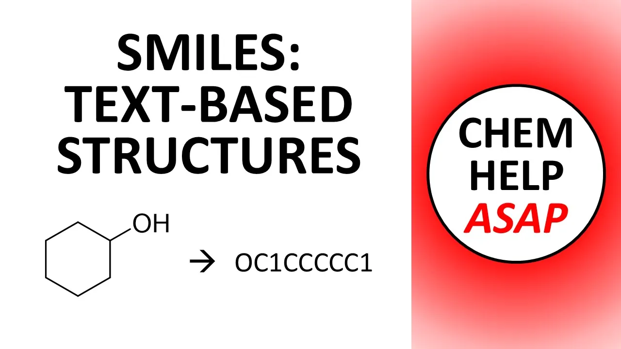
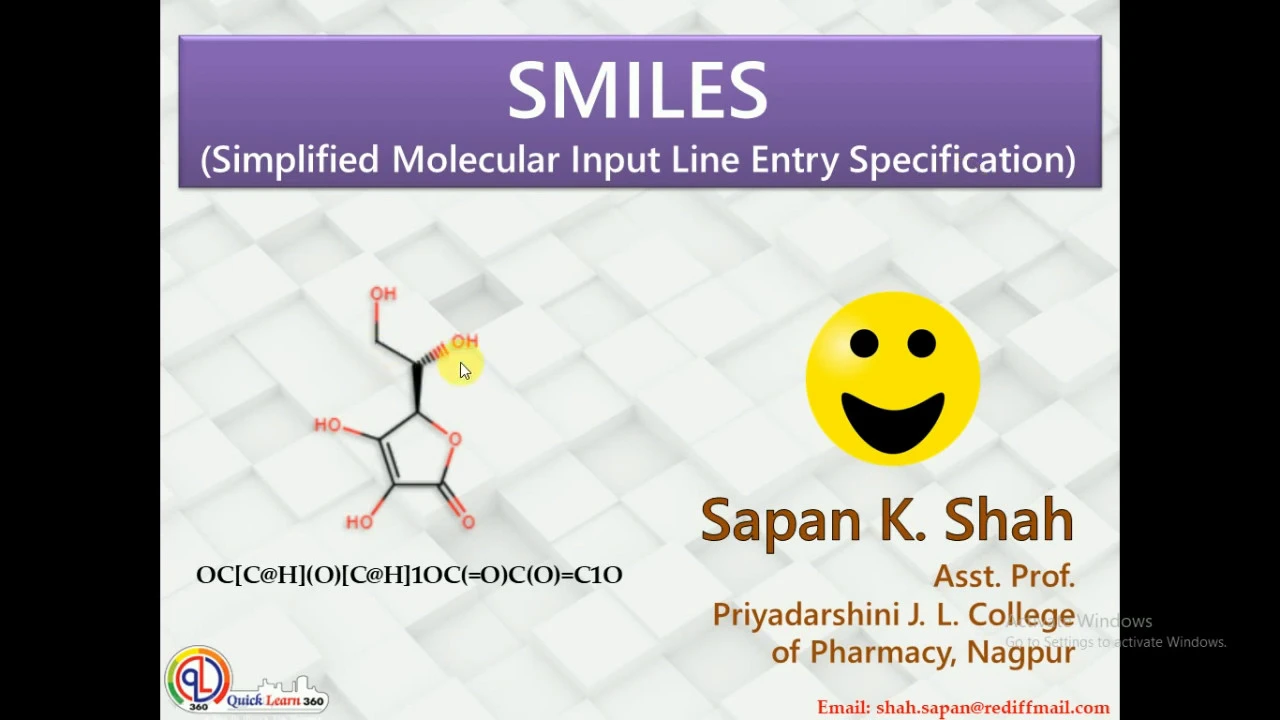
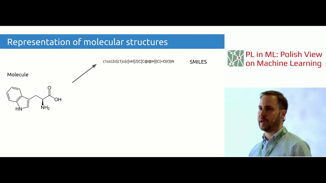
[00:00:01]so some of you have requested that I make a tutorial video about how I applied data science to my work and so in this tutorial I'm going to do just that I'm going to show you how I apply data science to the field of cheminformatics and in this notebook it will be a end-to-end machine learning project in Python and so we will be reproducing a published paper from de l'année who built a linear regression model for predicting the solubility of molecules so the solubility of molecules is an important physical chemical properties for drug discovery as performed by pharmaceutical companies and academia and so without further ado let's get started so the first thing that you want to do is head over to the github of the data professor click on the code repository find python and click on that and then scroll down to find chem informatics predicting solubility click on it and then click on the raw link right click save the ass and save it into your computer okay and if you want to follow along on google collab you can do so click on file open notebook click on the github tab type in data professor and then find chem informatics predicting solubility click on it but because I already have it open I'm going to use that and so here I'm going to clear all of the outputs by click on the edit clear all outputs so we're going to follow this along step by step so before beginning I got the inspiration for this Jupiter notebook from a excellent blog post that I read from Pat Walters so he is one of the authors of the deep learning for the life sciences book by O'Reilly and so the book was about the application of deep learning for predicting various activities and properties in the life sciences where he briefly discussed in the book about predicting the molecular solubility but a more in-depth example was provided by his blog post and so the data set was downloaded directly from the original paper by John de l'année ok so without further ado let's have a look at the code so the first thing that you want to do is you want to install our tee kits and in order to do that you need to install the Conda ok and the installation of Conda is already described by my previous video so if you haven't watched it yet please click on the link above okay so run this cell and so this cell will install Conda and then followed by the installation of the r/t kit and so this should take a while because our the kit is a pretty big package okay and now we have already kit installed already originally described the data set for the solubility of molecule was derived from this link and the original paper is linked here data was coming from this paper published in the year 2004 and so in this paper they predicted the lock s value the solubility value of compounds and so the supplementary file is right here if you click on this link or from the original article it is in the supplementary right here in the tabs so if you click on it it will be the exact same files that we have in here so we're gonna go ahead and download the data okay and then we're going to use pandas to load in the data set oh it was temporarily unavailable let's try again okay and so it's still not available so let me do this let me download this and then I'll upload it to the github of data professor so that doesn't work then we'll use this from directly from the github then okay and then I'll rename this to import pandas and then all we did and again okay now it works so feel free to use the version that I uploaded to the github just for backup purposes so as you can see that it didn't work on collab but it worked on my local computer okay okay so let's continue and read in the data set and which we have already done and let's print it out and so we can see that there are a total of four columns and the first column will be the compound name and second is the actual value the experimental value for the lock s the solubility and then the third column is the predicted value from their study and then the fourth column are the smiles notation and so in the field of chemistry Matic smiles notation represents the acronym for simplified molecular input line entry system and it is essentially compressing the chemical structure information into a one dimensional form and so the one dimensional form is shown here for example F would correspond to fluorine C will correspond to carbon n would correspond to nitrogen all would be oxygen equal sign would be double bond okay and the parenthesis will tell it that is attached to a particular atom okay and so we're going to use the smiles column and so we're gonna type in Sol which is the name of the data frame dot smiles and so we see the smiles column and it has a total of 1000 144 rolls or compounds and so if you want the first smiles from this list we're going to use the slice function so we're gonna type in so dot smiles bracket and then the number 0 for the first row and so if we have one here it will be the second compound and if you have two it will be the third compound etc and in order to allow the Artic kit to comprehend the information of the chemical structure we're going to need to read it in to our T kit by converting the smiles notation which is an ASCII text into a our ticket object so we're gonna use the chem sub-module dot mol from smiles function so what this essentially does is convert the smiles notation from the ASCII form into the objects okay and so we see that the object is right here and it this unique ID and it will be exactly the same as using the string of the smile siltation as I have shown earlier and I type in soda smiles bracket zero it will be giving this string as the output so you can also specify the smile string directly so either run this line or this line and you will see the same thing that the molecule will be generated and they will have a unique object ID okay and then we're gonna do this further by assigning this article object into the variable m and then we're gonna use some function to see how many number of atom does it have so we're gonna use M which represents the our ticket object for the molecule and then dots the function get number of atoms and so we're gonna see that this compound has six atoms okay so what this essentially does is it compute the number of atoms in the molecule and so we're gonna continue with calculating the molecular descriptors using the RT kids and so we can do this in the chem sub module so from our ticket import chem okay and so I'm gonna show you two methods of doing it and it is essentially the same thing the first method will be more lengthy we're gonna use the for loop in the original form and the method two will be the for loop but in a more concise way as you can see it is in the one line okay and so using either method one or two it will produce the same output so let's try with method one and so what does this essentially does is first it will create an empty list and for each of the smiles notation in the soda smiles list it will iterate for each element in the list of soda smiles it will convert the element into an RD kids object and then it will assign the article object of the molecule into the mol variable and then it will append the small object into the molar list variable list here that you see so it will start from a empty list and with each iteration each molecule from the soda smiles will be converted into the article object of the molecule and it will be appended to the mote list so this thing will grow okay and let's have look and so it has a length of 1144 which is the same number as the number of compounds and so let's show only the first five and so it will look like this so you see that there are five article objects here okay let's do it with method two and we're gonna call it a slightly different name more list two and 1144 compounds and the object as usual okay so now we have already converted the smiles notation from the text form into the article object form of the molecule and now we're going to continue with using the article object molecule in order to compute the descriptor and the original study by de l'année he made use of for molecular descriptors comprising of the optional water partition coefficient which is the ratio between the solubility of a molecule in optinal and water and so the lock P will be one of the descriptor to predict the lock s which is the solubility in water and the second descriptor is the molecular weights and so the molecular weight is the summation of the individual atomic weight and the third variable is the number of rotatable bonds so let me show you this this is a molecule and the rotatable Mon will mean like this how many bonds can be rotated as you can see the atoms were moved because I rotate the bond and if I rotate this bond right here right here in the gray color in a gray color if I rotate it notice that the atoms are moving see the red represents the oxygen black represents carbon white represents the hydrogen and so this bond is rotatable okay this bond is also rotatable okay and this bond is rotatable right here I rotate it but this double bond you will see it here this double bond it has one two it's a double bond it cannot be rotated okay okay let's continue and so the fourth descriptor is the aromatic proportion and this represents the ratio between the number of aromatic atoms to the total number of heavy atoms and so RT kit can readily compute the first three descriptor and the fourth descriptor we're going to have to compute that manually and so how are we going to do this exactly we're going to just manually compute the ratio between the number of aromatic atoms and the number of heavy atoms so just a simple division but we're going to have to manually compute each of these descriptor separately and then compute the ratio okay and so here we're going to compute the three descriptors locked P molecular weight and the rotatable bonds and so we're gonna use the article chem module and we're gonna import the descriptor function and so please note that this block of code was inspired by this cold ocean project here for the generating of the descriptors using the RT kits and so the first block here that you see in the function it will essentially do the same thing as I have already discussed up here in method 1 or method 2 or by it will create an empty list of the molecule and then read each smiles text and then convert that into the article object and append it one by one into the mold list okay and then here we're gonna just change the name or list to become more data so essentially it will convert the smiles text into the RT kit object and then after that it will compute the four descriptors using the mole object and so when the descriptors have been computed it will convert it into the numpy array and then it will dump it into the data frame using pandas and so it will return the pandas dataframe okay so let's run this block of code here and so let's generate the descriptor and put it into the new data frame variable okay I have to define the modules when it again all right so the descriptors for the first three are computed successfully and now let's proceed with computing the fourth descriptor the aromatic proportion so let's show you an example of how we compute this for a single molecule so for the M variable it's going to be the smiles of the molecule and then we're going to convert this into a our ticket mol object and so for the molecular object here we're going to retrieve all of the atom from the molecule and then for each atom we're going to determine whether it is aromatic or not aromatic and if it is aromatic it will become true and if it is not aromatic it will be false okay and then we're going to count the number of true and so that will give us the number of aromatic atoms okay true and false so true will be the number of aromatic atoms and so we're gonna count all the true here and so here it will be the summation here so let's we find this function and then let's determine the aromatic atoms in the molecule and then we have nineteen so the molecule up here there is nineteen aromatic atoms meaning that the atoms are belonging to the aromatic rings okay and so we're going to do this computing of the aromatic atoms for the entire data set so we have the number of aromatic atoms for each of the molecule okay and we're gonna do the same thing using this example for a single molecule and then we're gonna use the descriptors dot heavy atom counts in order to get the number of heavy atoms 19 and so the previous number aromatic atom is 19 and this heavy atom count is 34 so 19 divided by 34 will give us the ratio of the atomic proportion so we're gonna compute the heavy atom count for the entire data set and so we're gonna take in these two variables the aromatic atoms and the heavy atom count and then we're gonna divide them and so SEC 19 divided by 30 for the aromatic atoms divided by the heavy item count will be 0.55 88 and so we're going to do this for the entire data set and so here you go the aromatic proportion descriptor has already been calculated we're gonna combine the two data frames together the DF which contains the three molecular descriptor and the DF aromatic proportion which is the fourth molar descriptor so we're going to combine that using PD concat and then as argument we're going to have it in the bracket the first data frame which is DF and then the second data frame which is DF the ESC aromatic proportion and then we're gonna set access to be one because we're going to take the two data frame and join them side by side and then we're going to have four columns and so this will represent the X matrix and so we will use the X matrix and scikit-learn for the model building in order to predict the Y matrix which is the log S or the solubility of the molecule okay so it is this column the second column and so we're gonna select it by using the eye lock function and then colon and then comma one because we want to select only the second column and we're gonna select this by the index number okay let's do that and then we have the second column select it okay and now we already have the data matrices of x and y ready and now let's proceed with data splitting and we're gonna set the ratio to become 80/20 and then for the data splitting we're gonna use the screen test split from the SK learn model selection sub module okay and here we use x and y as the import argument and the test size to be zero point two because we want the test to be 20% and so the 80% will be the train set and so here we're gonna build a simple linear regression model and we're gonna assign model equal to linear model dot linear regression and then we're gonna have the model built using model fits and so the model dot fit will use the X variables and the y variable for model training and now that we have the trained model we will apply it to make the prediction on the extreme and the X test for comparative purpose okay and then we're going to run the model and then we're going to apply the model for the prediction now and so the first prediction we're doing here is on the X train data set and so this is for comparative purposes and then we're going to print out the coefficients and the intercept and in the metrics such as MSE and the coefficient of determination which is essentially the Pearson's correlation coefficient squared and now we're going to apply the model on the X test the 20% okay and we get the R square for the train set to be surplus 77 and the R square for the testing set to be 0.75 and so let's now have a look at the linear regression equation and so the equation provided by the work of de l'année provides the following equation lock s equal to the y-intercept 0.16 minus 0.63 c log p minus 0.006 - only her weights plus 0.06 6r b minus for AP okay so we see that there are the four descriptors and then the number in front are the regression coefficients which are right here and in the y intercept is right here and so let's compare that with the reproduction by Pat Walters and it is right here 0.26 for the y-intercept 0.74 for the LOC p zero point zero zero six six molecular weights zero point zero zero three four for the RB and 0.42 for the AP okay I noticed the positive and negative signs in front as well and so our notebook we production provide the following equation so at first glance it seemed that our model our B variable had a different sign for the regression coefficient but notice that this is for the train set and so the two studies here were based on the full data set and so we also compute the regression equation for the Foo data set as well below here and so we see that there is reasonably similar for the two equation by Pat Walters and the one by our notebook only with slight deviation for the rotatable bonds but the other are exactly the same point two six point seven four point zero three two but this is 0.03 four and the AP is exactly the same point four two okay and so here we use the full dataset to build the model so we're gonna run it and so notice that the equation that we have up here was provided by the following block of code so as always we use the modular string format to display the equation by taking in the variables as shown here after the percent operator and so the same equation can be generated using the following block of code and so the block of codes here are slightly easier to read because it breaks down each component into the individual variable intercept lock pmw RB and AP and then we use the modulo operator and then we're going to print it out by fusing together all of these and then we get the equation okay so these two block of code is essentially the same as this block of code here okay and then the equation that we got for the full dataset right here was derived from the run here just gonna run it equation let's paste it above okay and so let's have a quick look at how we can plot the scatter plot of the predicted value versus the experimental value and before doing that let's do a quick check of the variable dimensions and so for the training set we have 915 compounds and the test set we have 229 and let's make the scatter plot you see matplotlib and so we have this to plot and we're stacking in vertically we're asked in the following block of code we have it Oris on tally okay and so let's go into detail here and so we notice that we have two blocks of code right here the first block of code represents the first plot and then the second block of code here represents the second plot okay and I notice that here in PRT figure we define it to be the dimension of the figure so five is the width and so 11 is the length so we see that the weight is five and the length is 11 to accommodate two plots and in here we define the subplot one to be 2 1 1 and subplot 2 to be 2 1 2 and 2 the first number here 2 corresponds to 2 rolls and then the second value 1 it's one column and then the third value here 1 is the first plot and 2 is the second plot okay and so for the input argument of x and y in the plot scatter function we're going to use the white rain to be the EPS and then the Y predicted of the training set to be the Y and then we define the color and C argument here and then we make each of the data samples dot here to be having a transparency of 0.3 and then the trend line which we see as red color is provided by this block of code here and so we're using the numpy polyfill function and so the details of this was taken from the stack overflow here and so we're gonna plot the Y label and the X label correspondingly as you can see here we plotted once not here but only at the bottom and to the left okay and now let's jump onto the horizontal plot so the concept is exactly the same but notice that the subplot has two numbers be a rings a little bit it's now 1 2 1 before it was 2 1 1 & 2 1 2 because 2 was two roles one is one column and then we have 1 & 2 which is the plot 1 plot 2 but in here we have only one row so it starts with 1 and then the 2 here corresponds to 2 columns and then we have 1 & 2 which corresponds to plot 1 plot 2 ok and everything else is the same but notice that the x and y label here is slightly shifted in the above we have the F label to be occurring one time and we have Y label occurring two times okay here X label is occurring from one time for the bottom plot and the y label is occurring two times 1/2 because we have here one two and for the horizontal plot because we want to display the X label twice we're going to have the X label two times in the code and then we're going to have only the Y label once okay and then PLT does show to show the figure and then poto savefig to save the file into your working directory okay and so a less list and then we're going to see the created PDF and PNG files okay okay so congratulations you have now built your first kim informatics project by predicting the solubility of molecules and so here we reproduce the work by de l'année which he performed back in 2004 and so we have reproduced this using Python so I could learn and we visualize the distribution of the data points using the matplotlib so please feel free to modify this to be a different data set and as always upload it to your github and expand your data science portfolio because the best way to learn data science is by doing data science and so please enjoy the journey thank you for watching please like subscribe and share and I'll see you in the next one but in the meantime please check out these videos