














![[4] Óptica de rayos - Simulación multifísica en Ciencia e Ingeniería (5.5)](https://i.ytimg.com/vi/fkZ6-okCEjw/maxresdefault.jpg)



This webinar demonstrates how to model laser beam propagation in Zemax OpticStudio using two approaches: ray tracing for collimated laser beams (treating them as parallel rays) and physical optics propagation (POP) for Gaussian beams, which accounts for diffraction and wavefront distortions; the session covers Gaussian beam theory fundamentals including beam waist, Rayleigh range, and phase radius of curvature, followed by practical examples of designing a laser beam expander and optimizing a spatial filter to improve beam quality (M² factor) from approximately 1.4 to nearly 1.04.
Laser Photonics Modeling with OpticStudio: A Webinar Guide
Added:Fundamentals of Geometrical Optics: Understanding ray tracing, Snell's law, and thin/thick lens approximation equations.
Gaussian Beam Theory: Conceptual knowledge of laser beam propagation parameters, including beam waist, Rayleigh range, divergence angle, and the M-squared (M2) quality factor.
Wave Optics and Diffraction: Basic principles of wave propagation, diffraction limits, and how spatial filtering works in the Fourier plane.
Introduction to OpticStudio (Zemax): Basic familiarity with the software user interface, lens data editor, and coordinate systems.
Advanced Physical Optics Propagation (POP): Modeling complex diffraction effects, fiber coupling efficiency, and arbitrary phase plates or diffractive optical elements (DOEs).
Laser Resonator Cavity Design: Designing stable and unstable laser resonators, and calculating mode structures within the laser cavity.
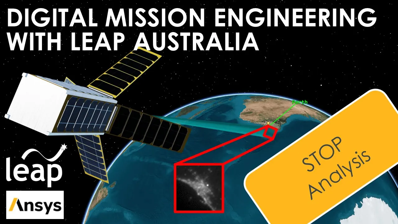
Thermal Lensing and STOP Analysis: Simulating thermal distortion in high-power laser optics using integrated Structural, Thermal, and Optical Performance analysis.
Tolerancing and Sensitivity Analysis: Learning how to perform tolerance analysis on laser collimation and focusing systems to assess manufacturing and alignment yield.
8.8K views68likes43:08Original Release: 2016-11-16
[Music] hello and welcome to this webinar on laser applications in zmax optic studio my name is Marc Nicholson and I'm going to be your guide for this this whole session in terms of user interface everything that we're going to be doing today or almost everything you're gonna find in the analyze tab of optic studio in the laser and fibers group we're gonna be looking at Gaussian beams and then physical optics in the beam found viewer we won't actually do much with the fiber coupling on this webinar that's covered elsewhere in other webinars and other knowledgebase articles first of off and as I saw a frequently asked question all the examples and these PowerPoint slides are in a zip file that we can mail to you after the webinar so don't worry about it you'll being able to keep up or take notes because we'll send you everything that you're seeing here today then the way that laser beams are often modeled is simply as collimated ray bundles and this works well in a lot of cases the trick is to know when it doesn't and that's really what this webinar is going to be discussing but for things like interferometers common path or shearing interferometers this is probably the most common application for the laser as collimated rave on approach and it basically treats the laser beam as if it was just a bundle of parallel rays and it's most commonly done using non-sequential ray tracing although it gets done in sequential as well and here's an example in retracing where we model a Mikaelson silencer promise er we have two windows here with 50/50 coatings on them we have two mirrors and one mirror is very slightly tilted with respect to the other and as a result when the beams recombine the overlap and interfere and we get fringes as a result of that as another example in one look shall just do a little bit more example on just think about a laser beam expander and this is a classic kind of thing that you would use rays for rays are coming in from the rear bundle that is a particular size over here there it is so the Rays coming in from its rear bundle over there and then it's going to another lens and then it's going into a beam splitter which is giving front and back reflections now this beam splitter is a little bit subtle and if we look at it in the editor you'll see that it's got a very slight so you can't really see it in terms of a visual layouts but if I just click on the back surface of the window and right mouse click I can scale it all of its properties and you can see here that the there is a very very slight wedge angle that's been placed in X on that so if you want to look at the same thing here you can do those just click on it here it shows you this in here so if you look at the front surface the front surface has no edge at all the back surface has this very slight edge angle and in terms of positioning is positioned at 45 degrees in the beam so we then take the reflections from front and back face and we interfere them and because of the X tilde interference fringes now if you see here you can see like two overlapping circles the degree of overlap is due to the thickness of the beam splitter but the the fringing is caused by the tilt angle of the back face of the shear plate and this is the beam perfectly kilometres we've got the the separation between these two systems is exactly what it ought to be and [Music] here we have it 205 if I make that 203 so that we the expander is slightly out of focus and the Bema is now enlarging slightly diverging if I repeat the retrace now then you can see how those fringes rotate and they rotate slightly clockwise if I put this language in two or seven and so at the expander or so that's slightly converging light affected by two or seven is slightly diverging lights and if I repeat the raytrace now you'll see the fringes rotate in the opposite direction and this is of course of a classic measurement technique for a laser beam expanders but this is just an example of modeling a laser beam in in zmax it just uses the individual rays we just coherent Li add them up works just fine in a really wide range of applications but but when de Rais not work and to understand that we have to think about Gaussian beans and then we'll also think about not not perfectly Gaussian beans I'm going to build a great example that demonstrates where simple retracing doesn't work and where we need to use physical optics and stand that's going to be a spatial filter with a non Gaussian beam being presented to us and a Gaussian beam being precisely uproot these soffits before we get there let's just think about what Gaussian beam Theory is Gaussian beams are an alternative to retracing it's a purely paraxial models and there's no aberrations considered by Gaussian beam theory and a Gaussian beam is defined by any two of three parameters wavelength clean waste and divergence and they're controlled by this expression and they're often used to study a tem zero zero perfect gaussian laser beam propagation and here's a schematic of what happens when you bring a Gaussian beam to focus and you'll see the key thing is that a Gaussian being cannot actually come to a point image it's not possible to produce a point image of a laser beam instead the smallest area that the beam will form is a region that we call the beam waist and by convention we refer to the waist as the half i'ts of the the being measured from the z equals zero points so that gives us a beam moist which is the minimum sports science that we can achieve the next concept is the Rayleigh range and the Rayleigh range is the distance over which the beam size has increased by root 2 times the beam waist or about 1.4 times the beam waist and you'll see that inside that really range the beam size is not a simple straight line now if you think of this as a point source with some divergence angle Omega or theta rather then at large Z distances the Gaussian beam does look like a point source and it's size increases linearly with distance but inside the Rayleigh range the size variation is more complicated and we refer to this one of the things we use to reverse this is the phase radius of curvature now the phase radius of curvature is infinite here at the really range in other words all you know if you were to differentiate the wave fronts everything would be pointing along this direction it comes to a minimum value at the Rayleigh range and then as you go off to infinity the phase radius of curvature goes infinite again and it's given by this expression and the Rayleigh range itself is given by this expression it just depends on the beam waist and the wavelength and this is what makes a Gaussian beam so interesting is that as you come to focus instead of just following the straight lines down to a point focus instead the wave front self interferes and it prevents a point focus from being formed and as a result we get the fundamental differences between rays and Gaussian beams rays always travel in a straight line and they can be brought to a point focus whereas a Gaussian beam doesn't really trim it clearly it travels in a straight line along the z axis but if you're if you're measuring the width of the beam within the Rayleigh range it does not scale linearly with distance and so Gaussian Gate beams diffract as they propagates and so the beam changes size and it's effective divergence as the beam propagates and then if we add in a thin lens with some power then we simply transform the radius of curvature it's given by this expression but we still maintain a spherical phase radius so new aberrations get added and this is where physical optics adds the capability to track aberrations as well as to add in diffraction from arbitrary apertures and people often think as a pop as being important because of the aberrations of bits right because of the apertures in the ability to handle a diffraction from our arbitrary aperture but it's really important when we look at laser beam propagation from the perspective of being able to see the phase distortion of the laser beam and as a result to see how M squared varies even though maybe nothing in the beam is actually a perjuring or clipping the game so we're going to do an example here and I'm going to start off with a helium-neon laser beam that is the red heaney lying beam divergence of 2.5 millimeters so beam diameter I beg your pardon 2.5 millimeters and our divergence of 0.1 75 million radians and then 10 millimeters after this laser there's going to be a 5 millimeter thick n bk7 lens the image plane is going to be 50 millimeters beyond that and our problem is to design the lens that gives the smallest Gaussian spot size at the image place and there's an important point here the beam diameter as the beam emerges from the output face of the laser is not to be confused with the beam waist typically the beam waist and the output port of the laser are two separate things so some resonator exotic designs do place the waste ass or near the output pores but they're not in general the same thing and typically they are the beam waist for a fabry-perot sight type of laser like that the helium neon tube laser the beam waist can be meters behind the output face of the laser and in the Gaussian beam calculation with an optics Tennille we always define the beam waist relative to surface 1 it doesn't happen to be surface number 1 we just have to position the waist relative to surface 1 so here's our first step we're going to define the laser I'm gonna do it like so I'm gonna actually open up one of the sample files that I'll be sending through to if you're interested this don't say that and it's simply this system setup I've given an entrance pupil diameter of six millimeters just so that we actually get some rays showing on the screen I'm the wavelength is set to the helium neon red line and I have defined surface number one to be the beam waist and I've defined surface number two to be the output port of the laser and that's you know that's almost it the the next thing to think about that it's hard to find the the Gaussian beam now the Gaussian beams being waste is completions with lambda and the tangent of the divergence angle and I get near one point one five millimeter value so the the waste is one point one five millimeters and the beam when it's emerging from the laser itself is one point two five millimeters so the beam has grown as its propagated and we need to compute what that distance is and so what I've done is I've set up the beam waste some distance from the output port and I want to see what kind of size the beam is as it as it propagates on the output face so to do that I'm going to go to my Gaussian beam paraxial Gaussian beam calculation and we're going to set it up like so I'll go set the waist size a 1.15 I'm going to make surface number one the waist so this surface one to waist distance is zero and I want to look at the beam size on surface number two which is the output force and you'll see that acts like a little calculator and it tells me that the waist is 1.15 millimeters its position is a hundred millimeters away if you see here and the beam size is just over 1.15 so I can I could play with this by hand and it'll make this 200 ever light and just have a look and see how much bigger they this the beam size gates are going a little bit bigger but not very much or I can do it the smarter way and have zmax I actually do the calculation for me so you can see I've set this up as a variable that's going to be for variable and just to be consistent with the north-south good I like to 100 and if I now go to the optimized tab and open up the merit function editor you can see what I've got in the merit function and it's a is an operand called Gbps Gaussian beam paraxial size and it starts at surface number two or it was set rather at surface number two the beam waist is 1.15 at a distance of 0 from surface 1 and I want to target the beam size to be one point two five zero millimeters and you can see that it's currently 1.15 all one three I'm only showing three decimal places yeah so all I need to do is optimize there's a start button the merit factor goes to effectively zero straight away and you can see here the distance that I have between the the beam waist and the output port you can see here that the the beam size is exactly one point two five millimeters at the output port five millimeters away it's growing by an additional three point four microns and just make this plot easier to look at I'm only going to draw from the output ports onwards now it just looks like like salt so that sets up my my beam weeks I'm going to take the variable off of that I'm gonna go back to the north and that just goes through exactly what we've covered I wouldn't talk through those slides it's just everything that we've done the automatic optimization another going to add the the lens and ten millimeters away from the output port is a five millimeter thick lens and then there's a 50 millimeter distance to an image surface so it's a model that I'm going to click on surface number three and pressed in certain cells gives me two surfaces that this is there that it's currently fine should actually be ten there should be a five millimeter and ek7 and this should then be fifty milliliters I just admit this to draw a little bit more easily the similar Amasa margin I'm setting to be one millimeter and they're just it just means that the importance on draw larger than the beam that's being drawn is and I've now fixed this number so I don't need to change it but what I want to do is optimize these two parameters so I make them variables of control Z and I'm going to go back to my merit function and instead of looking at surface number two I'm going to look at surface number five that being the final surface and instead of a target of 1.25 or what the service is zero I want the smallest spots I can have and if I just update that you'll see the meritocrat is no longer zero it's um it's actually it's the same as that the beam size if I just hit optimize start bang down it goes and I get a value of eight point three microns so you see here the beam size as it leaves the laser is one point two five millimeters but not as that lands on the surface the image surface it's eight point three microns so that's given me a nice focused laser spot on this laser this this lens would be would be very very good for focusing a lens like a laser like this one so again the notes just go through everything there but we've set the problem dosing beam calculations is that there's not much else you can do with this it gives you things like beam waist and phase radius really range in such way it works in spherical and cylindrical systems but it doesn't really give you any other useful information and it doesn't let me say how much wavefront distortion that winds has added to the laser so this is where physical optics comes in and I'm gonna set up physical optics that like so I'm gonna get myself in the north's to the same points as where I was and I'm gonna set up physical optics now to do the same calculation so I'm going to go back to analyze physical optics I'm just going to turn it off to apply off so that it doesn't apply as I'm as I'm talking because that could be useless and I'm gonna start the the beam at the beam waist I'm going to propagate it through to the image surface under being their condition I'm going to use a Gaussian waist and a sampling of 128 by 128 and the beam waist is going to be one point one five one point one five one point one five and then for the author old size of the array I'm just going to press the automatic button and that will size the array for me I'm going to tell it that I want to see a cross-section in X of the irradiance as a result of doing it and noticed that sort of one I'll apply that and there is my B min value there are four times zoom and let me just take that off apply that so there's there's my Gaussian beam on the image surface and you can see the pilot size is about eight point three microns of it you can just read that little part of the text there it says pilot sizes eight point three microns a nice looking Gaussian being but let me now show you the phase of the beam and here's the real reason for using physical optics is you can now see the distortion of the wave fronts of the beam as it goes through this lens and you can see a couple of things very very clearly here you can see here's the focus that's being introduced by this center of the lens you can see the spherical that's trying to compensate it as you get towards the edge of the lens and you can also see the goys shift which doesn't normally really do a whole lot they just a Pistons on the offsets the this is the phase of the center of the on the beam so I've just used physical optics very quickly there to propagate a Gaussian beam through the optical system and I've been able to see the irradiance and the phase of the beam as a results so it's really cool you can see all of that and by the end of this webinar you will know how to measure the M squared of this beam and I'm leaving that as a task for the for the viewer is once you get these sample files to measure the M squared of the beam after the webinar we're going to cover how to do that but what we're going to go on to now is a spatial filter and a spatial filter uses the lens to focus beam on so a pinhole the focal plane were effectively taking the Fourier transform of the complex amplitude of the beam the small pin or allows only a fundamental mode to pass and so the output is a ghost in intensity profile with some ball intensity rings around it and let's just have a look again I have a file setup for this that's example and here here it says it's two lenses they're a chromatic doublet and we use a chromatic doublet because the sensor surface is still used to control spherical so this is a very good imaging performance for an application like this you can see also from a point of view of the Rays I'm using a Gaussian app in ization just so that it looks more like a retrace and he looks more like a Gaussian beam when it's a trace but that done a man is going to hide the system Explorer it's not really relevant to us and let's just have a look at the physical optics propagation window and first of all I'm starting cancer plus one there's a that's that's my beam waist but surface one this time is defined as this donut beam and this is a multimode file I don't really have time to explain multimode files on this webinar but this is an addition of a TEM 1 0 and 0 1 mod and it gives me this kind of distribution a donut rifle ring with a zero of intensity at the center of it and then I'm propagating that all the way through the system in surface ones in the image displaying all the way through the system and you can see that I'm also saving the data on all surfaces so over here I have a beam file viewer and this is currently let me just make this larger you can see this is looking at surface number one and if I just give this one to the focus I'm using the left and right arrow keys and as I press those arrow key buttons the just need to make this oh sorry heritance I want to zoom in by a factor of four and now if I just use the right arrow key you'll see that I'm propagating surface by surface through the system so here I am now at surface five which is where the pinhole is going to go it isn't actually there yet so surface fine and surface 6 which are called locators look identical right now and you you probably can't see with the color resolution of the webinar software so let me just use a log scaling to show that the intensity actually goes out all this this way again if this book if this we're a go scene being you would expect to see a Gaussian focal plane but you're actually getting something much more complex than that if I just look at this as a cross-section in X you'll see that I'm getting a minimum intensity is around about 5.6 microns something like that and their intensity comes back up again and goes down it's my intention to spatially filter this beam so that we allow only the Gaussian portion of the beam above the fundamental mode through the system so let me then just go back to showing this as false color I'll take the log scaling off and then we just come back up and we propagate through the rest of the system there's the lenses and then we come to the final surface surface number 10 and we have reconstructed the donuts that we pre crusin so in other words we've pushed donuts in and we've got a donut out that's just talking us through everything that now sequins N squared factor is a great way of diagnosing beam quality and we can use it first of all as a diagnostic for any beam and also as a target for optimization and we the definition is that our beam with an M squared of 1 will change size as you propagate the same race as a TEM 0-0 Gaussian is and any other beam has an M Squared bigger than 1 and so that will refract faster than a perfect Gaussian beam would and M Squared is a so-called output characteristic the beam can't be defined by its M Squared so there's an infinite number of beams that have a waist of new 0.5 millimeters and then M squared of 1.3 so you can't uniquely define a beam with this N squared but you can measure the quality of any beam with its M Squared how do we get this well we get it using an optimization operon called pop D and science for physical optics propagation data and it returns all the beam characteristics that are required and it will give us things like the pilot beam day so the centroid locations effective widths M squared and x and y and and so on and so what we're going to do is to configure this is we're going to press the Save button on the pop settings dialog and that saves the current settings of the physical optics propagation calculation and then we're going to open up the merit function so let me just press save on here and then I'm going to open up the merit function and you'll see you have pre-built the merit function and it uses the pop D operand item 23 gives you the x width x and 24 gives you the wide width item 25 gives you the N squared and X and 2650 M squared and Y and of course as this is rotationally symmetric we expect them to be the same so we use it first of all looking at surface number one wavelength one and few long that's all there is in the system and we've got a beam width of one point four one four and x and y and an M Squared of one point four three one in x and y we then get the same data on surface ten and the beam is slightly larger it's a one point four one eight so it's only larger by four microns but the M Squared has no worsens and it's now about one point seven five three so that's the beam radius and M Squared just propagating through these because if nothing actually happening or have no pimple or anything like that in there yet so what we're going to do is we're going to add a pinhole at surface number five then I said it's aperture to be about five microns and I do that because when we looked at the irradiance if it minimized at about five microns and we want to as well as cut the beam down we also want to minimize the amount of diffraction that's introduced by the pinhole so that's why we're choosing a 5 micron distance so let me just go back to Z max optic studio and go back to the awareness day editor which is hiding here and on the surface number five which is the pinhole I'm going to double quick I'm going to go to the aperture tab and I'm going to sit on it a circular aperture with the maximum radius of point or all five that's five microns and I'll just click away from that and it will be accepted I don't know and if we repeat the physical optics propagation calculation now you'll see that the output beam has now become circular it's lost the door nuts that we were starting off with again let me just go back here to the starting I'm going to go through this surface by surface so there's the doughnut of the input beam and I propagate through surface two and then three focused through surface two and then three four and then I come down to surface number five which is now going to pinhole on it and if I just show this again as a cross-section cross-section in X I'll short the log feeling then you can see how the Beeman is being truncated right at that point and then I go on to surface number six which is you know call locator so the beam looks completely unchanged and so I'll just go back to my false color and linear scaling and you can see that as it propagates away from the the pinhole I've now got a central kind of lobe structure that comes up and was like so and here's now my output beam and when you look at the cross-section of the output beam cross-section in X and that looks much more like a Gaussian beam should look like remember I'm putting in that multimode distribution and I'm guessing out a distribution that looks Gaussian so just how good is it well let's have a look at the merit function again now that we've done that we recalculate the merit function you'll see that the N squared of this beam is now 1.25 so the N squared of the beam is now smaller than the M squared of the input beam so we've cleaned that beam up considerably the question is now can we actually make the M squared even better you know can we optimize the N squared and the answer that is yes we can the things that we want that the distance from the focusing lens to the pinhole so we can get that optimized for the starting distribution we get the tightest focus on the pinhole and then the size of the pinhole can be varied and our goal is to get the smallest m squared value so our variables are the thickness of surface for which is already I should may well have been set already yet so there's the thickness of surface for and then I also want to make the radius of this aperture that are placed on surface five variable and there's a sneaky way I can do that in principle its presence not an editor parameter it's not optimizable but I can cheat and I'm going to use the operands a key M X aperture maximum on surface number five I'm just going to make that a variable should be have you had it so I managed to sneak my pinhole aperture into a variable rather nicely I'm now I'm just going to go back to the merit function and all I need now is the minimum size of the beam on surface five and the minimum M squared on surface ten so let's just let me just do that right now so I'm going to go back sit here and I'm going to just delete all these off rounds I'm going to just insert a couple of new lines and I'm gonna get smallest beam on surface five as one of my goals I need that to be op deep surface number is surface number five wavelength as wavelength one feeling this field one the data item that I want on this is 23 that's the X radius I want to target that to zero with the weight of one and then I want smallest M Squared and chew on surface ten and to do that when it is popped D again but this time on surface ten is 1 1 again and this time I'm going to use parameter 25 which is the M Squared parameter and I'm going to target that to be 1 the weight of 1 so what is target is 0 make it as small as possible the other one is targeted to 1 because n square can only go to one and I'm not going to just call the optimizer and because I've only got two variables in here and they're both strongly couples I'm going to use the orthogonal descent optimizer I'm going to just use one cycle of optimization just for speed in this example I'm going to fire that off and listen take a few seconds if I took about 42 seconds it's going to exit from that update here and you'll see now that the N squared has improved to the value of one point all four so that is very very nearly a perfect Gaussian so I'm now getting a really nice gaussian out of this system not only does it look like a Gaussian but if I look at the fees going across it you can see that that's a far better looking fees distortion you can still see there's focus and spherical a little bit of Gouri shift as well but I've done a really good job in optimizing that M squared is coming just where I wanted it to being only just slightly greater than one so I've designed a really good spatial filter here I can also do things like I can tolerance the spatial filter and say well what happens if the pinball signs berries or happens with amount of focus and such I can and see how the M squared rather varies as a result of that but I don't have time to do that moment so there we go so in summary here razor a great first pass how these things behave but they do have some limitations paraxial gaussian beam adds extra information where ignores the aberrations and physical optics gives the best of both worlds when rays are not adequate because it lets you look at the phase profile of the beam and i've also actually quantify that in the most meaningful way that is used in laser physics which is by N squared so we discussed a shearing interferometer oops I'm just showed you how to use straight forward rays it's a bottle in that case the collimation of a laser beam worked perfectly we looks at a simple lens that we optimized for Gaussian beams and we've got some residual phase aberration when we use pop to look and then we used a spatial filter we could look at the input beams M Squared which was about 1.4 or something like that we just put a filter in and hoped for the best and that God is down to about 1.2 and then we optimized the system and that got us down to one point all four and M squared so you know physical optics when it comes to the design of laser optics optics user intended to image or focus or modify a beam very very powerful capability [Music]
Up Next
14:45
Simple Pendulum Period: Physics Tutorial
@khanacademyphysics7609
384.2K views•2016-07-29

12:53
21cm Hyperfine Transition in Neutral Hydrogen: Radio Astronomy Basics
@AaronRobertParsons
12.4K views•2011-10-13

32:32
NMR Spin Physics I: Zeeman Effect, Resonance Condition & Larmor Frequency
@nptel-indianinstituteofsci8064
2.3K views•2024-01-17

27:14
Entropy and the Second Law of Thermodynamics Explained
@veritasium
27.5M views•2023-07-01
Related Study Plans & Knowledge Roadmaps
Structured learning paths in Physics
physics
Nuclear Physics (Decay, Fission & Reactors)
01Atomic Structure and the Binding Force
02Radioactive Decay and Half-Life
03Nuclear Fission Mechanics and Chain Reactions
+ 2 more learning modules
12h5 modules
Explore Roadmap
physics
Soft Matter (Polymers, Colloids & Rheology)
01Foundations of Soft Matter & Thermal Forces
02Polymer Physics and Macromolecules
03Colloids, Surfactants, and Self-Assembly
+ 2 more learning modules
38h5 modules
Explore Roadmap
physics
Analytical Mechanics: Lagrangian & Hamiltonian
01Mathematical Foundations: Calculus of Variations
02From Newtonian Mechanics to Constraint Dynamics
03The Principle of Least Action & Lagrangian Mechanics
+ 3 more learning modules
28h6 modules
Explore Roadmap
physics
General Relativity (Spacetime & Cosmology)
01Foundations of Relativity: Special Relativity
02The Geometry of Spacetime: Equivalence Principle & Curvature
03Einstein's Field Equations: The Mathematics of Gravity
+ 2 more learning modules
55h5 modules
Explore Roadmap