




















![[ICRA/Forums] Compliant and Precise Control of Humanoid Robots](https://i.ytimg.com/vi_webp/dU0KhBL91vM/maxresdefault.webp)
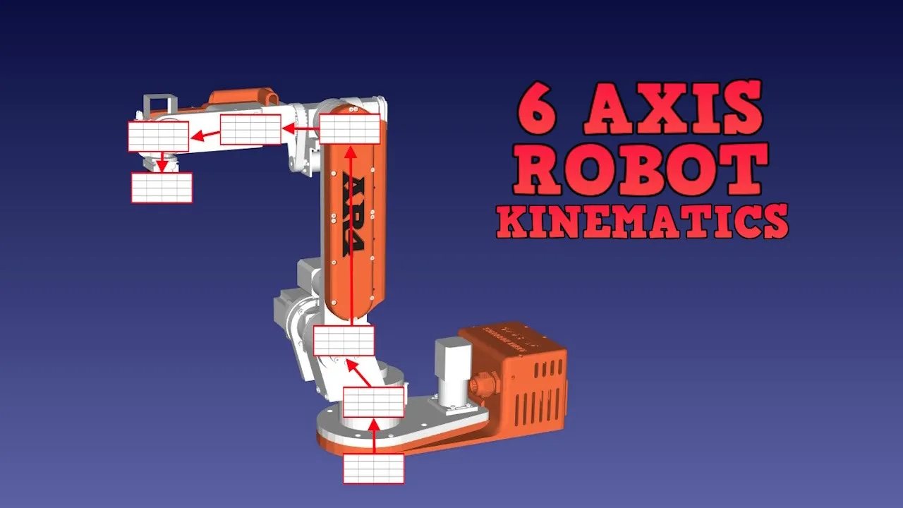
Inverse kinematics determines the joint angles required to achieve a desired end-effector position in robotic systems, and there are four main approaches to solving this problem: explicit (manually deriving and solving equations), hybrid (combining symbolic and numerical methods), implicit (using the model itself as the inverse solver), and pure inverse model (where the entire model is inverted to compute joint positions directly from desired end-effector coordinates); the choice of approach depends on the system complexity, computational efficiency requirements, and whether the system has redundant degrees of freedom.
Inverse Kinematics for Industrial Robots and Manipulators
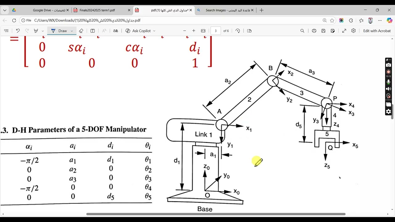
Added:Fundamental concepts of Forward Kinematics and Denavit-Hartenberg (D-H) parameters for defining robot configurations.
Linear algebra, specifically vector calculus, rotation matrices, and homogeneous transformation matrices.
Basic numerical analysis and root-finding algorithms (e.g., Newton-Raphson) used for solving non-linear systems of equations.
Familiarity with symbolic mathematical computation tools and multi-domain physical modeling environments.
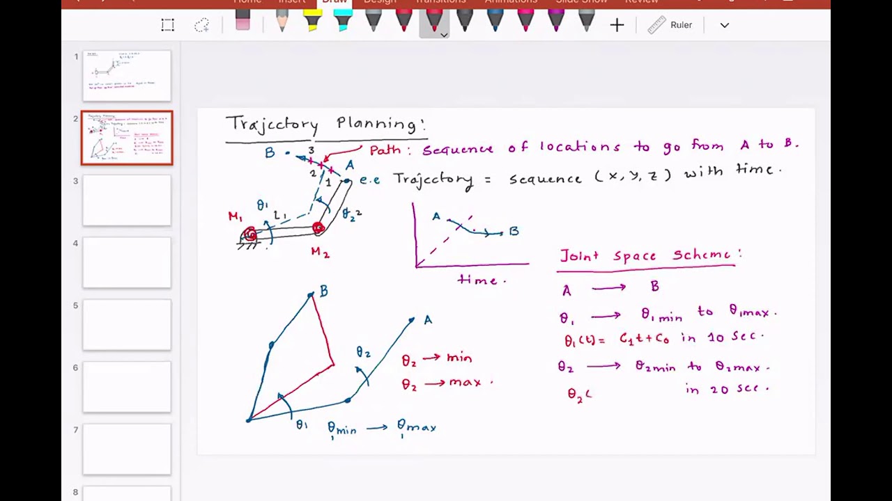
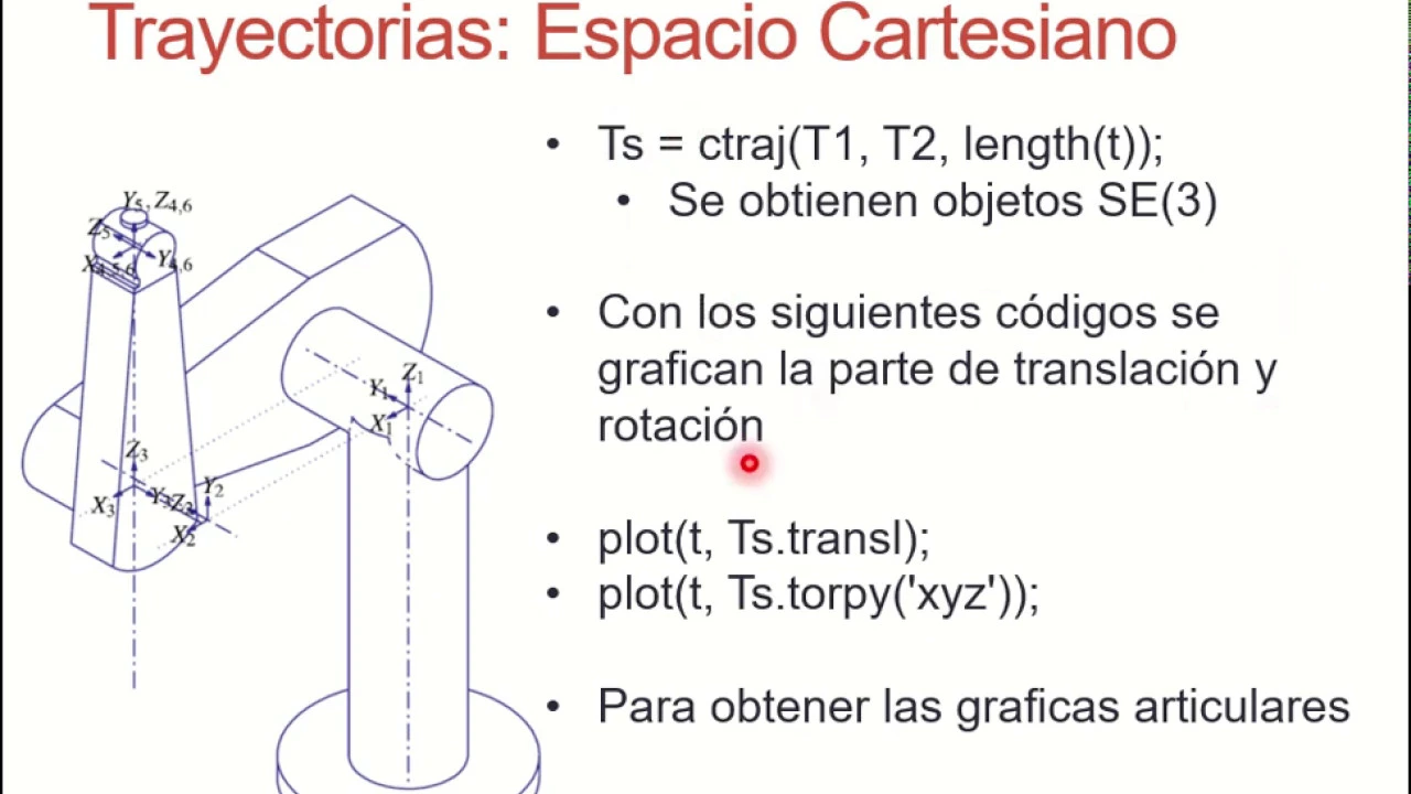
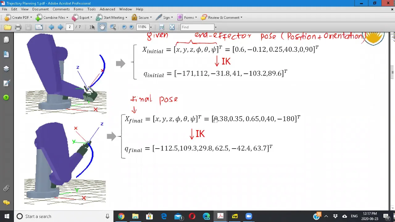
Trajectory planning and Cartesian space path generation, translating continuous paths into joint space coordinates over time.
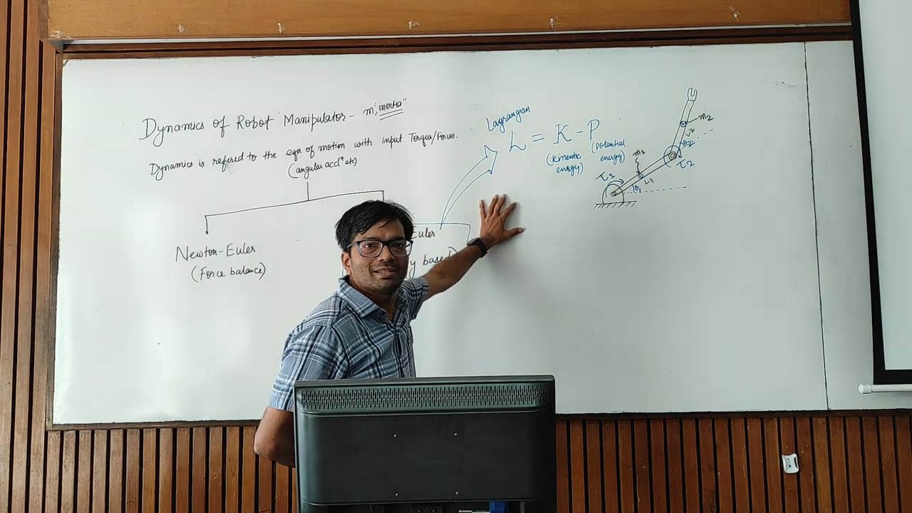
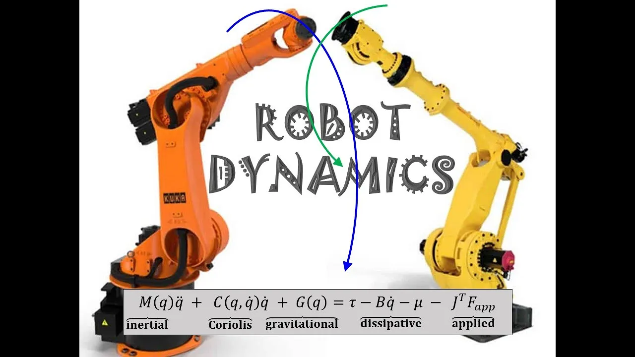
Robot manipulator dynamics, exploring how forces and torques relate to kinematic motion using Lagrangian or Newton-Euler formulations.
Singularity analysis and avoidance techniques to manage configurations where inverse kinematics solutions become unstable.
Real-time code generation and deployment of kinematic algorithms onto industrial PLCs or robotic controllers.
Advanced elastic-joint and flexible-link modeling to implement active vibration control in high-speed precision tasks.
2.4K views16likes57:41Original Release: 2022-02-22
[Music] and welcome to this session on inverse kinematics in industrial robots and manipulators so i'm going to get us started [Music] i have put together a number of examples as rachel mentioned those are provided in the download link that has been shared with you in the chat so it would be great if you guys can um download and um try to follow along um so um before we begin um let's start i want to talk a little bit about the the motivation behind this um session uh we've been working uh a lot with our cost uh our customers on on the variety of uh projects that would require some aspect of inverse kinematics custom robotics cnc machines the driving simulator hydraulically actuated booms like the ones that are mounted on a truck so these are the type of applications that we have been involved in and our technologies are very well suited for uh so that that gave us the inspiration to put together this uh session on inverse kinematics this session will not be a a complete treatment of the subject this would be from our point of view and where our technologies and our approaches have have practical use cases uh so in in particular we will not be i will not be talking about um iterative or jacobian based approaches uh i'm gonna for the most part stick to square systems uh so the redundant systems will not be covered there are some expect exceptions and this session will not be touching on trajectory planning or optimization topics but i will cover as i mentioned would be square systems where we have the same number of actuated degrees of actuated joints and degrees of freedom for the end effector we'll see examples of both open and close kinematic chains uh we'll have uh a special extension to the inverse kinematics for flexibility and this is specifically for um compensating the effect of gravity on the linkage which could be a a topic of concern for especially large manipulators and as we have covered in previous [Music] workshops in this series we'll talk about cable robots as well so let's uh let's very briefly talk about inverse kinematics so first forward kinematics in forward kinematics we go from joint space to cartesian space where we have the value for the actuated joints like this simple pictures we have theta one and theta two and we want to find where the end effector is or the x and y which is usually a simplest straightforward problem to solve and we plug in numbers to the equations and get the values the the inverse of that which is the topic of this session is is much more complicated involves many different numerical and numerical approach to get to the solutions and there are sometimes no solutions some most cases multiple solutions that that can can come out of uh solving those nonlinear equations um so that's that's the that's the premise that's uh the area that we are going to be talking about but as i mentioned this is not a treatment of the topic this is taken from applications that our technology has has been tried and and is is been been utilized so let's have a look at the scope of what i'm going to be covering today um just to put some context we're talking about getting some equations that these equations would be are what we want to solve to get to the inverse kinematics of of the system the robot the manipulator um so then so then first is the derivation of where the where the equations come from the process of solving them and then putting them into a component um and then putting it in a in a bigger system model to simulate or in a lot of cases um in in control or automation uh the next step would be uh not only simulation would be to export so that this can be incorporated in the in the control code so the one approach is explicit is pretty straightforward where we have the equations we write them down ourselves or we use maple or a combination of maple maple same to get to those equations we'll see how that that that would work uh where we use uh just use maple and its symbolic computation capabilities or we use maple maplesim to drive those equations for us and then give it to maple for uh symbolic manipulation and attempt at solving this obviously could be just manual we have the solution or we use maple symbolic computation cable do that for us then we will package that in a component uh usually there is a translation between maple to modelica this could be explicit where you have to tweak the code and we'll see example of that or it could be done behind the scene by a command in maple that will generate the component for us put it in maplesim is another block and put it on canvas connect it up and we do the simulation the um the one that is uh maybe not as direct as the first category is hybrid and um hybrid means that we don't solve everything uh we might not be able to solve the equations so we leave some of them unsolved and let the maple same engine deal with those nonlinear constraint equations and this can continue to all the way to not solving any of the equations so we just generate the equation package them in a component and pass it on to maplesim for generation or export and we'll see examples of that as well and the easiest more straightforward most straightforward approach is just no equations at all where we use the uh inverse of the model itself as our inverse kinematic um so that that that approach is uh can can be used in a in a variety of cases and as i mentioned it would be the the fastest easier way to to accomplish an inverse kinematic of a given system and in some cases this could be one of the few choices so obviously not all approaches are created equal in terms of reach and the type of system that they can cover but also in terms of efficiency and how much work it is to get to them so i i put this qualitative graph um in in together to give you an idea of these main approaches so on the on the horizontal axis we have the complexity of generation as in how much work you need to do uh the expertise level that you need to have uh to to get to those um those solutions and on the vertical axis we have the computational efficiency so the more work you do to get to the solved set of equations um then the overall computational efficiency would be higher and that should not come as a surprise um then then we have um the inverse models uh there's a there's in a lot of cases when we are in maplesim and we want to use the or create the inverse model we can do some simplification to help us uh with uh i mean simplified in a lot of cases are better and also provides uh some uh computational boost the the good uh so so so the the simplification obviously varies uh depending on the case and we'll see examples of uh how how that would work uh and uh what type of simplification we're talking about uh in terms of between implicit and explicit also there is a range and depends on how much of the equations you can divide and conquer and and get to a solution for the good news is that as i said not only simulation but also the um in automation of control would be the the use users of this um these inverse kinematics solutions uh and so you you there is there's usually a required performance in terms of efficiency of calculation and how fast they run but the good news is in in many cases that we come across uh even the inverse model uh would be uh way past the um the requirements so we we don't need to worry about that too much obviously the more complicated the model becomes the more computational problem you need and then other approaches could be make that difference as i mentioned there is a little bit of a special addition to the implicit approach that i hope that i get to as one of my examples where we expand the implicit approach to creating an inverse kinematic block that also includes the compensation for the effect of gravity for that i'll convert a hydraulic actuator articulated boom to have one one piece flexible and then drive the equations some of the some of the topics that we are about to cover can be very technical um hope that you still find uh the the the the examples useful um and uh give you an idea of how these technologies work uh these are all created custom for there's no universal solution aside from the inverse model that you just package the model and it has a wider coverage when we get to equations it is case-by-case basis but i hope that i would be able to give you the workflow from equations to inverse kinematics so i i'll be jumping from the um the the presentation to maple same and maple and back so let's let's start with our first example so a warm-up a well-known robotic system deltabot for this one we are going to use an explicit approach and we'll just drive equations for the kinematic constraints in maple pretty straightforward for the delta bot and then use maple to solve those equations once we have the solution we'll grab those equations put them in a component um using the um the both maple and maple same metallic code editor and then hook everything up as you see on the screen and simulate the system so with that i am going to jump to uh maple sim here we go so here's uh for for those who haven't seen the product uh the the tool uh here's the modeling environment and we have on the left our library of various components and there's a message console on the bottom and the properties of components that we select on the right and in the middle of the canvas is where the blocks are put together so i'm just going to go and open the first example which you also have in the in the package that has been shared uh with you in the download link so just uh while i'm talking about that i'm going to run this as well so we have various blocks on the screen as you can see so the the lower part is just for completing the model and it's currently disabled we have the fixed base we have the three arms that are actuated by ideal motion drivers the the end effector and the connecting rods for the end effector what i'm doing here is simulating the model you can see that the inverse the inverse schematic block already is on the canvas so this model is pretty much finished we'll have others uh other examples as we go forward that that might not be as as complete as this one so let's take a look at the animation first so we are executing a command we're going one third of a full circle and then execute a pick and place we'll come back and run this simulation again uh with with the with the grippers as well but uh let's let's uh go to the the main topic of uh this example so in maple syme um as we will see uh over and over again in the uh reminder of this session you will have additional information that you can include with your maple sym model and those are usually found under the attachments in this case under the attachment we have a maple worksheet for deltabot inverse kinematics and we can open that by double clicking on that so it will open maple and so here is basically a calculation sheet uh where i have uh typed in the equations and uh use maple to solve them so i'm just gonna zoom in a little bit i'm not gonna spend too much time on the actual derivation here because this is previous standard you basically uh go from the center point of your end effector and write the full basically the the vector from this point to uh this point at the end of the arm and we know the length of that um that vector and we calculate that length so that will give us one equations uh for theta uh which is our which arm angle so that's the that's the equation that we need to solve to get the relationship between where our end effector is and the angle theta one theta two theta three so here is just a vector notation of um the the positions and calculating the norm of that and basically equating it to l2 which is that linked and this is the constraint equation that we want to set to 0 and solve looking at it we have the coefficient for cosine coefficient for sine and whatever remains that not function of theta so it's really um becomes a a cosine plus b sine plus a constant and we can have maple solve that you have two solutions we know which one we want to pick so at this point um in this example everything is done manually i've seen the equations i have the definition of a b and c uh what i have done in this model is created a medical custom component and i have the solution as you just saw in that maple worksheet just put it here and the definition for a b and c that i'm passing to this function that i've created so the reason i've created this function is that as you remember we have solved it for one of the legs and we just can use the same solution for all the legs and then we put them all together in a modelica custom component generate that and that becomes this component that we use to actuate the system so this one is is almost entirely manual aside from the assist from maple to solve that equation and give us in a in a very uh nice uh format so that we can uh we can use it uh but we will see that for more complicated and uh more bigger systems um the the manual approach might might not be very convenient uh so we will use uh maple to generate the modelica for us instead of or at least parts of it uh as as you will see in the examples so um last thing on this example is just to complete it with uh giving it the grippers so that it will pick up the balls and put them in on the on the ground uh so it uses the some other libraries in maple sym the multibody library and uh the the pieces in there would be the grippers the the proximity sensor and also the contact library okay so that's that's our example number one our first uh warm-up example so we now go to our second warm-up example i'm going to go back to the presentation and look at the example number two the example number two is the very well known squad platform uh we even simplify that further to three degree of freedom basically um confine the platform to um to translation only the next example would be the full sixth degree of freedom it's just a because we're going to dive into equations this this seemed like better suited for the purpose of this session this one is also explicit approach where the only difference really the previous one is that in the previous one we know how to drive the constraint equation here we let maple api to maplesim to extract those equations from the model and then do the the rest of the process using maple to solve and then putting them all together again in maple and simulating so let's let's go back to maple syn open the second example it is go up one example number two i'm just going to open this um so here is the uh second example also uh completed uh so this is the expected configuration of the stored platform with uh six legs um we have uh some sample commands for how we want the to platform to move i'm just gonna run this while i'll uh describe the model uh if we go the the the legs are identical uh they are parameterized so they all place in the right location at the right angle but the equation inside them or the configuration inside is identical each one includes its own inverse kinematic block that receives the um demanded or required platform position as an input and calculates the length of the corresponding leg um that gets actuated by in this case a ideal position driver but this could be also a hydraulic system that gets this command from the inverse kinematics the inside the the leg we have the universal joint at the bottom to the ground the prismatic in the middle and the shoulder is a spherical joint so there's a number of degrees of freedom here that that form each of the legs so here is the simulation of the system the the yellow ones are the universal joints and the balls on top are the spherical joints and due to the inverse kinematic that has already been implemented the platform executes the commanded motion perfectly so let's uh let's take a look at how this inverse kinematic is created similar to what we saw in the previous example the inverse kinematic calculation worksheet is already attached this is just a maple worksheet you can have maple worksheets that do other types of work uh analysis preprocessing post processing here obviously we are concerned with worksheets that do inverse kinematic work for us um and there's a custom component that generated at the end under custom components and that custom component is the equation for this block here and we will we'll come across a lot of these as we go forward so just like before i'm going to double click on this maple worksheet to open it up um so here we try to go a little bit slower this time um so the the first command this is an active session this uh this maple worksheet is looking at the open vapor sim model so um the the first command establishes a link and creates a module a and then we will uh use that module a to create the multibody module and uh that's uh that's fair as as you're ready there multibody has some very nice structures in it and that can be utilized so here's uh zoom out first to see all the system the generalized coordinates the generalized the first and second derivatives of the velocity and acceleration coordinates and the reactions to the all-day constraints in the system it also reports that the system is modeled with 24 um generous coordinates and 18 so six remains but we'll we'll throw away another tree so that we deal only with uh uh with uh with translation so one thing that uh is first established here is that the leg equations are the same uh so what is what is happening here is that we get the position constraints uh for the system from the multibody object and the first three are for one leg then the second three is for the next leg and so on so we'll just pick two of them we use the same variables in both and subtract them uh from each other the leg one constraints minus leg two constraints and let's maples simplify the resulting expression which is zero zero zero so this is just a just a test to see that we can actually tackle one leg at a time and here what we are doing is creating the looking at one of the legs in a more generalized way so these are the um the the constraint equations uh for one of the legs um that has the um the what we want and some other variables that we might not necessarily need but we need to solve for it to get to the extension of the legs which is really this guy that we are after but there are other uh variables that we need to solve for so we can take a look at uh saying that uh for these um for these three constraints that we get what variable present presents in which one and how we can strategize a solving approach so we can see that we can solve the second equation for alpha because it's only function of the unknown alpha and the known platform position so that can be solved directly and then we can use alpha and beta we can use the first equation to calculate beta which we also don't need but we need it for the third equation to solve for s so that's exactly what we do first solve for alpha and then beta and then solve for s now that we have the equations that we want so together these uh this equation represent the solution uh we use uh the other api in in maple to maplesome and have that generate the modelica uh directly for us um and once that material is generated we'll just set it into the maple sim model this one was already there so it says that you want to overwrite which is the same same component that existed and it will give us in our local component section the inverse kinematic so this one was explicit but almost entirely automated from the getting the equations we did some checks and balances but then we were off to a fast uh continuation with generating the equations that we want we put it back uh and uh we we were able to simulate the system as we wanted so that's um kind of concludes our second warm-up example and we are at the halfway point so um i'm gonna be unfortunately speeding up a little bit more as i've already uh this was a very quick review of these examples so let's move on to our third example and the third example is again a steward platform but this is the first time we've been looking at an inverse model as i said this is the most straightforward way of modeling there's a little bit of a change in the in the model um the swat platform model and uh for a good reason because we're going to reuse the pieces back in maple sim uh so let's jump to maplesim and see how this was done so go back file open example number number three open that up so here we have the model here we have a fixed space base and then we have the moving platform and they're arranged um as a switch platform is arranged and what we are doing in the inverse kinematic block uh if i go inside by double clicking i'll see this you'll see the the same two pieces for the moving part and the fixed part which are exactly used in the inverse model and the difference is there is no dynamics here there is no degrees of freedom we are grabbing the um the platform and rotating it and moving it according to our command inputs so this is a prescribed translation and this is a prescribed rotation so six degree of freedom we are grabbing the the end effector of our inverse kinematic inverse model and moving it and instead of having the leg degrees of freedom the universal joint the spherical joint the prismatic all of that we throw them out and replace them with a sensor which basically uh measures the distance between the two ends of each leg there is some offset that you need to apply if there is an offset between them but basically this is your inverse kinematic solution so this disqualifies in if you recall from the big table this is an inverse model that is somewhat simplified we could have left everything there but this is a very easy simplification to draw out the legs and replace them with just a distance sensor and they're they're brought to the boundary of the component and that's our inverse kinematic uh just like the previous inverse kinematics block that you have seen we just hook everything up together and simulate and as we will see that there is there is really no difference between um this this block and the previous blocks in terms of the usage in maple syn code generation and other types of downstream applications um so um this uh this represents a potential um convenient approach to get to inverse kinematics for some uh difficult problems and um the last example uh that i have is a particular example of such case that that that the inverse model uh proves to be very very useful so as you can see i can command the the platform to do exactly what i want in sixth degree of freedom so compared to the previous example when we go to maple and generate the equations uh had to do some checking and then finding out what equation includes what unknown variable come up with the strategy of solving them and then proceeding to solve them and putting together uh back into a component this is a lot easier uh but again as we saw in that in that graph that i showed um that might be our starting point but uh for certain cases we might need to uh try to do something more efficient to hit our calculation budget when we are thinking about um the application on plcs or controllers that we want to put this on so but um but this is uh as as we have uh shown and used in applications with our customers this is still a viable choice in a number of uh situation and part of that comes from the core technologies of uh maple syn and maple where we use symbolic math to um to create a very very optimized set of equations for uh solving whether being a nonlinear solve here or any other solution um so that's that's part of the reason we we might be able to um meet the computation budget even with an inverse model so move on to my fourth example where things uh potentially get a little bit more complicated uh we look at our um a um first large uh manipulator system this is um as you will recognize from the from the the setup is inspired by some of the um truck mounted um the hydraulic articulated booms that are used in variety of applications so here we um we simplify the system to only um translation uh there's there's nothing stopping us from uh having a five degree or six degree of freedom five is more common in this type of applications um to do the same but because we're gonna go into the equations and do some um some more advanced stuff i felt like a 3d graph freedom would be sufficient so this one is implicit which means that we are going to generate the equations using maple and maple syn but we will not attempt to solve them so the process would involve building the model of generating symbolics extracting and then after the extractions we won't be able to put them all in one command and generate the custom component we actually need to put the pieces together and do some manipulation of the extracted modelica pieces and then create the inverse block and the rest obviously is the same as the previous examples so let's see how that would look like for this one i think i've i've included multiple um pieces so let me just go to fort folder example number four so we have a start finish and detour so let's start with start here and this this model that says um articulated boom start is really not for simulation this is our preparation for extracting the equations that we want uh so this the system is in place all the degrees of freedom is in place we have the rotating base we have the uh first uh revolute joint uh for the first boom and the hydraulic or the linear actuation in this case and the second linear actuation uh and the second uh second piece of our articulated boom um as we have seen before uh we'll just go to maple where the magic happens um i will go through this um again or step by step so we'll have some familiarity with uh with this we already saw some of these um so first step would be to establish the connection and the second step would be uh we do a lot of stuff with multibody so uh get that multi-body module which is very helpful in extracting variety of different things that we will see shortly this this this step could take a a bit of time to put that together that that module the good thing is that this is only in the in the generation part of our uh our path to the inverse kinematic uh we won't be doing this uh again after we have created the inverse kinematic block um so uh while that is happening i can i can explain uh what the next step would be uh the the equations are generated uh in in multibody with the system parameters left symbolic uh in this case we don't want to do that we want to get rid of those those parameters so we ask maple to or the maple to maplesim api to get all the parameters of the system to us and um once that is done okay this is finished uh it says uh five um degree of freedom or five um generalized coordinates uh the system is three degree of freedom so there's constraints involved two of them um the as i said get the get the parameters um so that we can substitute them away uh as we generating the the pieces that we want so one of the good things that that we get from that multibody is the gate frame motion basically we can find the vector to any point in our multibody in a symbolic form symbolic parametric form in general but in this case we'll substitute away the the parameters so that we we will get the the expression without any parameters so that's the vector where the end effector is and we also have a target for the end effector and all we need to do is set an equal to each other so right there i have created three constraint equations or three equations that i need to solve to find the um to to find the uh this the solution and i can the uh when i when i but when i look at these um equations um as you saw in the in the beginning uh only interested in um in in really theta one and if i go back here i'm interested in theta one uh for r1 and s1 and s2 i'm not interested in theta two theta three theta four theta five and so on so i'm not done yet the work is not done although i have created three equations we have the position constraints that we come across in the previous one so we grab those as well just like the previous one we'll take a look at see what's inside the position constraints uh our relationship between r3 r4 and r5 we'll we'll add them to the list of equations that we want to solve so we set them to zero and add them to the pile as second batch of equations so the the first batch was the end effector equal to the target the second batch would be the position constraint and as i said we are not interested in all the thetas be interested in the distances so we calculate those um separately or after the fact because right now we have five equations already of five unknowns so we can calculate r1 r2 r3 r4 r5 so based on r3 r4 and r5 we can calculate another one or two we can calculate the the lengths of the cylinders which would be the actual uh value that will drive our controller our hydraulic system and what have so for that we again go to get frame motion and say give us a vector from the start to end of cylinder one give us a vector uh from a start to end of cylinder two and we'll just keep them as um as variables in the generated metallica for the entire system we put everything together in one list of equations and use the maple to medical command to just convert that to a temporary medellin this is not done we still have to massage that to make it ready there could have been pieces that i can include here to do that but i felt like it would be more straightforward to uh to do that directly inside the editor so if you're going to folder for example number four you will see the the generated equations so this is what what comes up out of that maple to modelica command we have all the equations that we want uh the the the constraint equations the end effector equations and the xyz for the um start to end of our um our cylinders these are very large equations um that uh we have the uh luxury of having maple generate them for us and we don't need to worry about that so what i have done uh is that i do some um mix and match and let me just close this other ones that we'll get to hopefully so i'll do some change of variables add some additional pieces so if you go back you can see the inverse kinematic complete which i have used modelica and i can actually in my case i have the the coding so this will be better so i've added the inputs outputs i have the end effector as an input to my inverse kinematic i have the ground motion as an input to my inverse kinematic uh it could be on a boat it could be on a truck a set that the base could move and if we have those information the dangerous kinematic can compensate for and at the end although i have some other pieces that i don't want but i have to calculate the outputs that i assign to my inverse kinematic would be only the ones that i want which is r1 theta s1 and s2 um and really the only additional calculation that i would add is that i convert those length vectors to actual sorry the displacement from end to end of a cylinder to an actual length of the cylinders this um this code is grabbed and put in maple syn so the way i do that uh let me go back ctrl a ctrl c and i go back to maple sam go to code editor and put a blank modelica paste it and then generate the component for my maple syrup model so that completes the um the inverse kinematic uh generation for my maple syn model we have the completed model so i'm just going to switch to that i encourage you to try to finish that yourself to get to this part so now we have the commands uh some some paths that i have provided some disturbance of the base or the motion of the base and i'm also tracking the or plotting where the end effector is i want to excuse me make sure the end effector is following the path that i want um so in this case um let's let's uh once the simulation is over uh we can we can take a look at the the the system you can see that these the the cylinders are driven by the um [Music] like an ideal uh position drivers as i mentioned before this could be a hydraulically actuated system using our hydraulics library uh like the the inverse kinematic and directional control valve and controllers are come together to actuate the system we do have examples in that area i'm not covering them in this session but if you're interested in knowing more do do contact us and we can we can talk about those examples as well so i'm just simulating this for for 10 seconds let's have a quick look at the results so although the the base is uh obviously moving uh the uh end effector or or the points of that v based on calculation are clearly only uh covering the uh the commanded path so this is a this is a successful implementation of inverse kinematic uh for a uh articulated boom on a mobile system with moving base so the the the complication that we can add here is what if this system also because it's big so you can imagine and depending on the application if the application actually requires um more stringent error tracking when the operator says move forward up left down or rotate um you want to have more more accuracy you might need to compensate for the effect of uh inevitable effect of gravity on the the system so um and that's that's something that our approach of implicit equations and solving could also um come to play there as well so that's that's what i have uh for my next um example but before i go there i almost um forgot about the detour so the detour is i'm not going to run this but i'm just going to show it very quickly here what i've done here there is no inverse kinematic but basically what what i've done here is grab the end of the boom and move it so this whole thing is the inverse kinematic for the system you see that there is no actuation here and i'm reading as i'm probing the the three values that i'm interested in so you can imagine this uh whole system can be put into a block and exported as a code where it receives the base displacement the end effector desired position and the output would be exactly what we want so this is the starting point of a complete inverse approach to create inverse model approach to english schematics for this system i thought that i include that to give you a perspective of one version with respect to another so let me just close this and go back to our list of examples uh so example number five there there are more pieces here obviously with the uh with the inverse kinematics um there there are more pieces to look at so let me start with the finish then i will show you the the the pieces that needs to go together to make this happen this looks similar to the previous example i'm going to run that while i describe it uh but just for for the sake of simplicity uh i've removed the base motion there was there's really nothing prevents us from including those type of uh inputs here as well so um the this is the same system as the previous one except that for the last boom the last segment of that i've replaced the the original which was rigid with one of our flexible beams from the multibody library and even i can include multiple um deflection modes i've only included the vertical or the elastic coordinates for that direction um the the flexible beams in maple sym uh use um um shape functions and um as a solution to the partial differential equations that describe the a flexible beam so by a by including the number of terms you control the accuracy two is a very good guess for a lot of applications for involving beams um and uh i've only included two terms and there will be two additional variable associated with this um formulation of a of a flexible beam you might have a passive joint added to your system which has uh linear stiffness and damping and you want to you want to include that as part of your lumped flexibility the approach that is presented here can uh can account for that as well and the extra equations will be generated for the steadier state deflection due to gravity which will be joined to the part of implicit equations and solve all together for for the solution to work as as one unit so here let's take a look hopefully the the the flexibility of the top beam will uh will be visible in the in the in the demo so this i've actually included a very large mass at the end so that we can we can see the um the deflection uh but even with the deflection the ik is able to adjust the other degrees of freedom such that the um the end effector uh traces the exact path as commanded there are dynamic effects that are not accounted for and in a lot of cases uh these type of manipulators are not moving that very fast so this approach contributes to a much better accuracy of tracking and positioning for these type of manipulators as you can see here so this is these degrees of freedom are going to be different than what it was for the rigid case um to to get to these uh set of equations we actually have to uh create two uh models um i won't go to a lot of details um for that so we have two uh prep models uh that we need to put together i've also included a rigid comparison so that you can you can compare what would what would a rigid version of this system would look like how much extra joint motions are being applied from the ik to compensate for the flexibility and so on so part one of our preparation to generate the inverse kinematics is pretty much the same as what we have seen in the in the last one uh again i have the maple worksheets i'm just going to have a quick look but the difference between this one and the previous one is that when we do the steps um there is going to be two additional um variables that we don't have any ways for solving and those variables corresponds to the the flexibility of the beam um [Music] i'm going to escape that because i'm running out of time to get to those two equations um we use the part two of of our prep work so let me just open the part 2 and this one is a bit different as you can see we thrown out all the linkages we only kept the the degrees of freedoms that uh that correspond to the configuration of our robot nothing else or manipulator and uh for uh for the way we're generating the equations we have removed the revolut joints and prismatic ones with motion drivers so we can command the system to be exactly where we want and we left the obviously the flexible beam in place so this one is very different uh so we we basically generate the equations for this system differently um again as before we uh let me see if i can run this i'm just going to comment this out um so um as before we established a link but here we just go straight to the overall equations of the system with the git equations a command to get the all the order differential equations of the system and we get a list of variables that exist in these equations or the system and we will see that those variables are going to be the uh flexure variables of our beam and the next line here in equation three what is what happens here is that we zoom out a little bit now that we have the results there's only two variables the deflection variables for our beam and we'll set everything all derivatives to zero so we get a city of state equations and we can generate that uh to modelica uh i have included the two pieces generated in the in the folder as well so let's have a quick look at those uh so we have the two pieces equation one which is very similar to what we have seen in the previous example um except that you will see that these equations are function of these uh these variables as well uh see let's see if we can find them there we are so they are here and we need to solve for them and if we go to the second set that we are able to generate we create two equations that are uh for these these two additional variables this is the acidia state deflection on the gravity what we do we'll put them all together as very similar to what we have done again in the previous example and there we have the inputs and outputs we combine all these equations together so we have the the balance the component with the right number of equations and not right number of unknowns the same and just like uh previous time we calculate s1 and s2 and although we have some additional variables that we we don't need we have we calculate everything just like before we put these all together in our in our component a custom component and generate the inverse kinematic block so this is an extension of the implicit approach with uh with the gravity compensation and i felt like i should include that in this in this session because that's uh somewhat uh unique in in a way we we do that and seamless uh in the approach compared to what the previous uh step was to be able to use maple and maple syringe to generate the equations put it together and then put back in the model so there's there's very little time left uh thankfully the last example does not involve any any real work uh with uh with maple syn because uh i've already uh created an fmu for that i mentioned that the at the beginning that uh in a lot of cases uh the the end goal is to uh be able to generate the english kinematic in do a code generation on that not just simulation and uh so i'm just moving forward the last one here so this is uh this is again an inverse model but instead of uh running it at the end in maple syn we're running that in maplesome insight which allows us to run fmu's that are generated by maple sim that have inside information embedded uh so this is an inverse model so as i will show very quickly uh is we have this complicated robotic system and we want to find what each of these winches should command for this box in the middle to have 6 degree of freedom you can imagine writing the equation for this is quite a task but the inverse approach makes really short work of this system and really we we put a copy of the entire system back in the inverse kinematic and we are able to co-generate that and run it and to kind of get a sense of the efficiency of that calculation i have created a shared with you an fmu of the entire system not only the inverse kinematic part but uh the um the uh the the the robot itself so on on your side uh you need to find the um the insight application and run it and then use the file open to open the fmu from the provided files once you do that you get this view of the robotic system uh this is the exported fmu from maplesim so it's already generated equations optimized and all of that are done and we can go ahead and run the fmu so if if i run that one more time you see that the the pulleys are all oriented immediately at the start now we are ready to um because we have included some tunable parameters in this fmu command the system to execute and you can see that we are comfortably able to run this model um in in in a in real time uh fashion so we are commanding this to go at x y z and uh let's let's rotate this uh this is in radians so almost 90 degrees we can go further than that so this is this is a this is an idea kind of try to um establish the fact that this this approaches that we are talking about here even the most expensive one can be can be co-generated and be part of a a a a real use case you
Up Next

25:04
Designing a Quadruped Robot Leg: Inverse Kinematics and 3D Printing Guide
@TazerTechnical
8K views•2025-09-15

58:25
MathWorks Virtual RoboSub Simulation Environment | Webinar 2026
@RoboNationInc
209 views•2026-03-10

11:04
How to Build a Self-Balancing Robot: Arduino Nano & MPU6050
@easytechzones
16.8K views•2022-03-09
25:22
Micromouse: The Fastest Maze-Solving Robots on Earth
@veritasium
23.5M views•2023-05-24
Related Study Plans & Knowledge Roadmaps
Structured learning paths in Robotics
robotics
Building Delta Robots: Kinematics & Pico
01Foundations of Delta Robots & Mechanical Design
02Electronics and Microcontroller Setup with Pi Pico
03Delta Robot Kinematics and Coordinate Math
+ 3 more learning modules
65h6 modules
Explore Roadmap
robotics
Building Ballbots: Dynamics, Kalman & LQR
01Embedded Electronics & Omniwheel Actuation
02Ballbot Kinematics & Rigid Body Dynamics
03IMU Sensors & Kalman Filter State Estimation
+ 2 more learning modules
42h5 modules
Explore Roadmap
robotics
Micromouse: Hardware, PID Control & Flood-Fill
01Electronics & Teensy Microcontroller Basics
02Sensors and Actuators: Motors, Encoders & IR
03Precision Movement: Implementing PID Control
+ 2 more learning modules
35h5 modules
Explore Roadmap
robotics
CDPR: Kinematics, Arduino & Winch Control
01Foundations of Arduino & Basic Electronics
02Stepper Motors and Winch Mechanics
03Kinematics of 2D Cable-Driven Robots
+ 2 more learning modules
28h5 modules
Explore Roadmap