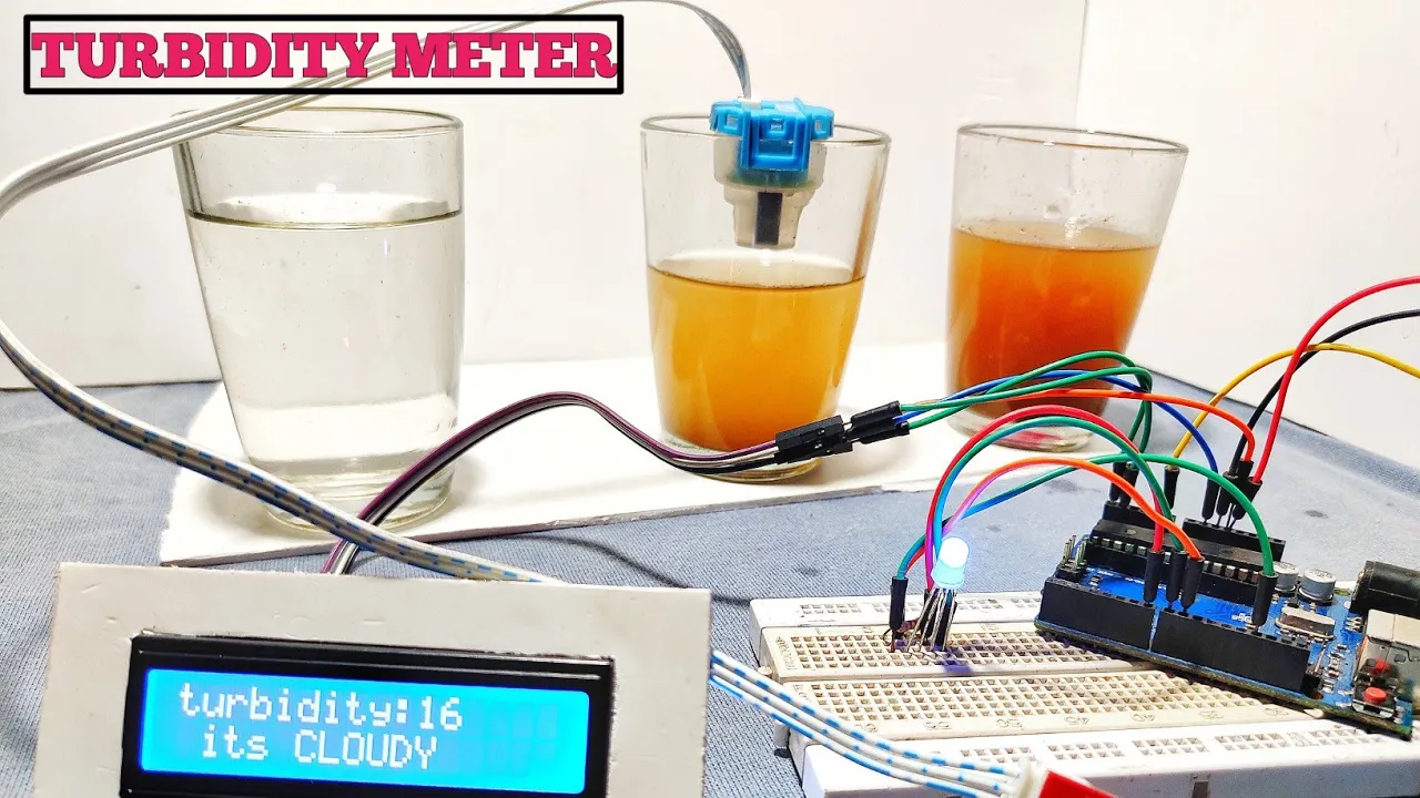
This tutorial demonstrates how to build a turbidity meter using an Arduino Uno and a turbidity sensor module, including the calibration process where you connect the sensor to Arduino's A0 pin, upload the analog read serial code, apply blocking material to determine the maximum turbidity value, then integrate an OLED display and RGB LED for visual output by replacing the default value in the code with your calibrated maximum reading.
Turbidity Meter with Arduino Uno: DIY Calibration & Build Guide
Added:Deep Dive
Basic Arduino programming and circuit design, including handling analog and digital I/O pins.

Podstawy Arduino, Odczyt Pinów Cyfrowych i Analogowych w Arduino, digitalRead, analogRead
1.3K
This segment covers the complete process of designing input circuits for Arduino. Digital inputs use a switch with a 10kΩ pull-up resistor between the pin and +5V, reading HIGH when open and LOW when closed. Analog inputs use a potentiometer connected to A0, with one side to +5V and the other to ground, producing variable voltage from 0-5V. In code, pins are defined using constants (PIN_BUTTON = 2) or A0-A5 notation, which Arduino maps to actual pin numbers (A0=14). The pinMode(INPUT) function configures pins for reading signals. Serial communication is initialized with Serial.begin(9600) for data transmission to the Serial Monitor.
Click to watch →

2Arduino
624
This tutorial covers Arduino's digital and analog input/output operations: digital pins use pinMode() to configure as INPUT or OUTPUT, digitalRead() reads HIGH/LOW values, and digitalWrite() controls LED states; PWM (Pulse Width Modulation) enables analog-like output through duty cycles (0-255 values) for LED fading effects; analogRead() reads sensor values (0-1023) from pins like LDR light sensors, which can be used to control LED behavior based on environmental conditions.
Click to watch →

Pemrograman Arduino Part 4 (digital Input/Output, simulasi tombol pada sebuah lampu LED pushbutton)
1.4K
Arduino digital I/O uses binary values (1/0) for on/off states. Digital output sends HIGH (5V/on) or LOW (0V/off) signals to control devices like LEDs. Digital input reads signals from components. To configure pins, use pinMode(INPUT) or pinMode(OUTPUT). Variables store data with naming rules: no spaces, max 32 characters, no reserved keywords. The IF statement creates conditional logic: if (condition) { statement1; } else { statement2; }. Arduino circuits require proper connections: power (5V/GND), push buttons with pull-up resistors, LEDs with current-limiting resistors. Breadboard traces connect horizontally left-right and vertically top-bottom. LED cathode connects to GND, anode to positive through resistor.
Click to watch →
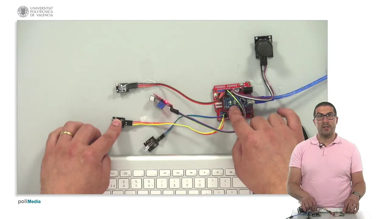
Facilino. Instrucciones E/S básicas. | 17/76 | UPV
721
Arduino handles two types of signals: analog (0-5V, converted to 0-1023 values) and digital (0V/5V, binary true/false). Analog reading uses analogRead() on pins A0-A7, returning 0-1023 values. Analog output uses PWM via analogWrite() on pins marked with ~, accepting 0-255 values (0V-5V). Digital operations include digitalRead() for input, digitalWrite() for output, and pinMode() for configuration (INPUT, OUTPUT, INPUT_PULLUP). Buttons read as HIGH when released, LOW when pressed.
Click to watch →

How to Program Arduino? Digital and Analog I/O l Getting started with your Arduino projects | Part 4
119
Arduino programming requires mastering digital I/O functions (pinMode, digitalWrite, digitalRead) for controlling digital signals and analog I/O functions (analogRead, analogWrite, analogReference) for handling variable voltage levels; digital pins operate with LOW/HIGH states while analog pins use PWM values from 0-255 for controlling devices like LEDs, with reference voltages determining the input range for accurate readings.
Click to watch →
Deep Dive
The physical concept of turbidity and how optical sensors measure suspended solids via light scattering (Nephelometry).

Nepheloturbidometry || Nephelometry & Turbidimetry || P4 Unit 2 || IMA 7th Sem || Carewell Pharma
116.7K
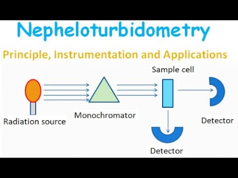
Nephelometry is based on the scattering of light by non-transparent particles in a suspension. When light passes through a suspension, the solid particles cause the light to scatter in all directions. The intensity of this scattered light at a 90-degree angle is directly proportional to the concentration of suspended particles. This technique is particularly suitable for low-concentration suspensions where scattering is minimal and manageable to measure.
Click to watch →

DIY Turbidity Meter using Arduino & Analog Turbidity Sensor
64K
Turbidity is the measurement of cloudiness or clarity in liquids caused by suspended particles that scatter light; it is measured using optical sensors that detect scattered light at 90 degrees, with higher particle concentrations producing greater scattering and thus higher turbidity values (measured in Nephelometric Turbidity Units, NTU), and the sensor output can be interfaced with microcontrollers like Arduino to calculate and display turbidity levels for water quality monitoring applications.
Click to watch →
Nepheloturbidometry - Principle, instrumentation and applications
41.3K
Nepheloturbidometry detects suspended particles through light scattering. When light passes through a semi-transparent medium, it undergoes reflection, absorption, transmission, and scattering. Homogeneous solutions show minimal scattering (4% reflection), but suspended particles cause significant scattering proportional to their concentration. The Tyndall effect describes this scattering phenomenon. Two analytical approaches exist: turbidimetry measures transmitted light intensity (inversely proportional to particle concentration), while nephelometry measures scattered light intensity (directly proportional to particle concentration). For accurate analysis, samples require insoluble, fine particles that don't settle quickly and are free of dust interference.
Click to watch →

Turbidity Measurement
222.5K
A nephelometer measures turbidity by detecting dispersed light. When light falls on the sample, part of it strikes the suspended particles and gets dispersed. The magnitude of this dispersed light is measured by the detector. The instrument has three controls: a range switch to select appropriate range based on expected turbidity value, and set zero and calibrate knobs for instrument calibration.
Click to watch →

Turbidimetría y Nefelometría
198
Turbidimetry and nephelometry are analytical techniques based on light scattering by suspended particles. Solutions (particles <1 nm) are homogeneous with no visible light scattering. Colloidal dispersions (1-100 nm) show the Tyndall effect where light becomes visible. Suspensions (>100 nm) are heterogeneous with easily distinguishable components. Turbidity is the cloudiness caused by light scattering from suspended particles. Transmittance (T = I/I₀) measures the ratio of transmitted to incident light intensity. The turbidity coefficient (A = -log₁₀T) quantifies scattering on a logarithmic scale. The turbidity equation A = K × B × C shows turbidity is proportional to particle concentration, path length, and a constant dependent on particle type, size, shape, and wavelength. Turbidimetry measures transmitted light in a straight line, suitable for higher concentrations. Nephelometry measures scattered light at 90 degrees, more sensitive for low concentrations. Tungsten filament lamps are standard light sources, emitting radiation from approximately 350-1100 nm. Standard turbidimeters operate at 400-600 nm (visible light). Wavelength selectors (filters) reduce the broad emission spectrum to the desired range.
Click to watch →
Deep Dive
Understanding the I2C communication protocol, which is typically used to interface with OLED displays.
Tutorial OLED I2C Display degan Arduino (Image & Animation) #Arduino
21.2K
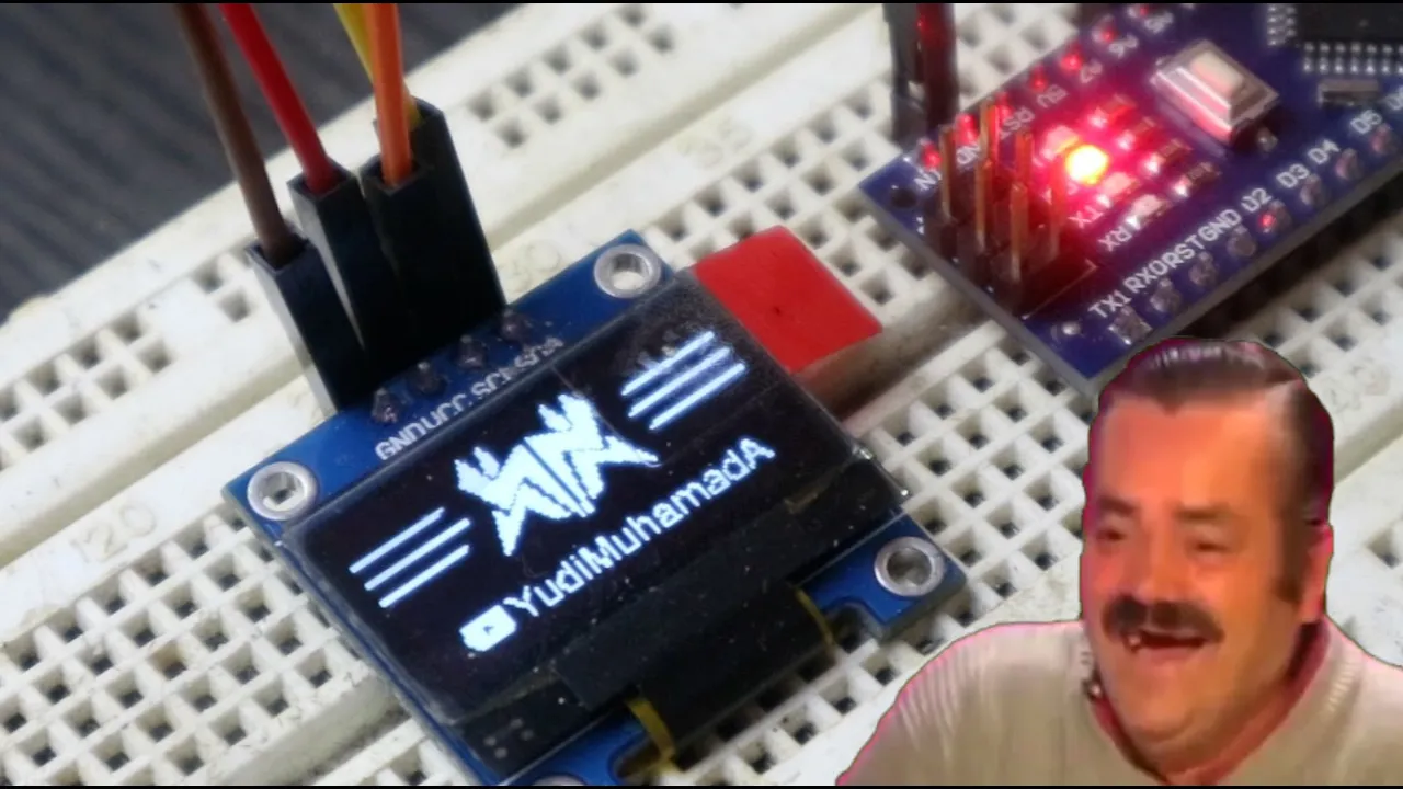
This tutorial demonstrates how to interface an OLED display (SSD1306, 128x64 resolution) with Arduino using the I2C communication protocol. The video covers hardware connections (GND, VCC, SDA, SCL), library installation (Adafruit GFX and Adafruit SSD1306), address configuration (converting 8-bit to 7-bit address), and essential display functions including display.begin(), display.clear(), display.drawPixel(), display.drawRect(), display.fillRect(), display.setTextSize(), display.setTextColor(), display.setCursor(), and display.drawBitmap(). The tutorial also explains how to create animations by converting GIF images into individual frames using online tools and implementing them in Arduino code with sequential display and delay functions.
Click to watch →

" Salidas Digitales de Arduino con Tecnología I2C y Pantalla OLED | Tutorial en Vivo"
449
I2C (Inter-Integrated Circuit) is a two-wire serial communication protocol using SCL (clock) and SDA (data) lines. In this architecture, the Arduino acts as master controller while the OLED display functions as slave device. The master initiates data transfers and specifies the slave address. OLED displays contain internal electronics that multiplex signals to drive individual pixels. This master-slave relationship enables simple communication requiring only two pins, dramatically reducing wiring complexity compared to parallel interfaces. The protocol allows multiple devices to share the same bus, making it ideal for connecting various peripherals to microcontrollers.
Click to watch →
Arduino + OLED = 3D ?
689.9K
The SSD1306 OLED display uses I2C communication protocol, which requires specific pins on the Arduino board. For hardware I2C connection, the Arduino Uno uses pins A4 (SDA - data line) and A5 (SCL - clock line). These pins are pre-configured in the u8g library for the standard I2C connection. If software I2C is used instead, any other digital pins can be utilized, but this method is slower than hardware I2C.
Click to watch →

Circuit 4A: SparkFun Inventor's Kit for MicroPython
201
An OLED (Organic Light Emitting Diode) display is a visual output device that uses a grid of pixels to display text and images by turning individual pixels on or off; it communicates with microcontrollers using the I2C protocol, which transmits data over two wires using binary signals (high for 1, low for 0) to send messages between devices, and the Qwiic connector system simplifies connections by combining power, ground, and communication signals into a single cable.
Click to watch →

Analog Clock using OLED Display with Arduino Uno Microcontroller (DIY)
159
This comprehensive section explains the I2C communication protocol used in the project. I2C uses two wires: SDA for data and SCL for clock signals. The communication operates in half-duplex mode, allowing data to flow in one direction at a time—similar to walkie-talkie radios where one party transmits while the other receives. The Arduino Uno serves as the master device, initiating all data transfers, while the OLED display acts as the slave device responding to commands. The SSD1306 display driver enables graphics and animations, requiring the U8G library for implementation. The OLED technology produces self-emissive light without needing a separate backlight, enabling thin, high-contrast displays with a resolution of 128x64 pixels.
Click to watch →
Deep Dive
Fundamental concepts of sensor calibration, specifically mapping raw analog voltage values to meaningful physical units.

Siemens LOGO! 8 - Analogwertverarbeitung
49.9K
LOGO! analog inputs return raw values of 0-1000 corresponding to the full signal range. Scaling converts these values to meaningful physical units using gain and offset parameters. Gain represents the multiplication factor (e.g., 0.2 for converting 10V to 100 units). Offset represents the null-point shift (e.g., -100 for a temperature sensor where 0V equals -100°C). The formula is: Physical Value = (Raw Value × Gain) + Offset. For example, converting 0-10V (0-1000 raw) to -100°C to +100°C requires gain = 0.2 and offset = -100. At 0V: 0×0.2 + (-100) = -100°C; at 10V: 1000×0.2 + (-100) = 100°C.
Click to watch →

Proyecto Final: Estación de clima virtual en tinkercad
247
Convert raw sensor values (0-1023) to meaningful units using formulas or MAP function. For soil moisture: (rawValue / maxValue) × 100. Test your specific sensor to determine its actual range, as different sensors produce different output ranges. The MAP function simplifies conversion: MAP(value, fromMin, fromMax, toMin, toMax). Always verify conversion accuracy by testing at minimum, middle, and maximum values.
Click to watch →
ساخت دستگاه فلومتر (Flow Meter) آموزش کامل به همراه کد برنامه نویسی
3.8K
Raw analog values from sensors (0-1023) need to be mapped to meaningful physical units. The mapping function converts the raw ADC value to a scaled value (e.g., 0-5000) based on known reference points. Calibration involves setting two reference points: the minimum value (0V) and maximum value (5V) that correspond to known physical quantities. This allows the system to display accurate, calibrated readings.
Click to watch →
Making Sense of Your Sensors
254
This section defines sensor calibration as the process of teaching a sensory system to convert raw voltage readings into meaningful physical units. It explains why calibration is essential for meaningful data collection and big data applications in agriculture. The linear calibration process is demonstrated using a pressure sensor example, where known reference values establish a mathematical relationship described by the equation y = mx + b. The slope (m) represents the voltage change per unit of the measured quantity, while the intercept (b) accounts for any offset. This linear mapping enables accurate conversion from sensor output to actual physical measurements.
Click to watch →

S6 E9. Electronic Fuel injection for the 212 Predator! it works! Can it really be this simple?
29.7K
Raw analog sensor readings from devices like MAP sensors are initially provided in counts (the ADC output). To convert these counts to meaningful engineering units (such as kilopascals or inches of mercury), calibration data specific to the sensor must be applied. The conversion formula typically uses the relationship: Voltage = (Counts × Reference Voltage) / Maximum Count Value. Additional sensor-specific calibration factors may be required to translate voltage readings into pressure measurements accurately.
Click to watch →
Prerequisite Knowledge
- Concept 01Basic Arduino programming and circuit design, including handling analog and digital I/O pins.
- Concept 02The physical concept of turbidity and how optical sensors measure suspended solids via light scattering (Nephelometry).
- Concept 03Understanding the I2C communication protocol, which is typically used to interface with OLED displays.
- Concept 04Fundamental concepts of sensor calibration, specifically mapping raw analog voltage values to meaningful physical units.
Subsequent Learning
- Step 01Developing advanced calibration curves using polynomial regression to convert voltage accurately to Nephelometric Turbidity Units (NTU).
- Step 02Implementing digital signal processing techniques, such as moving average or Kalman filters, to reduce sensor noise in turbulent water.
- Step 03Integrating the turbidity meter into an IoT network (using ESP32 or Wi-Fi shields) for real-time remote environmental monitoring.
- Step 04Designing a multi-parameter water quality monitoring station by adding pH, temperature, and electrical conductivity (EC) sensors.
Calibration
Build Meter
Calibration
0:00Playing Section
- 1
Connect sensor to Arduino and measure baseline values.
- 2
Apply blockage to record maximum turbidity reading.
- 3
Store calibrated value for meter configuration.
Limitations of DIY Turbidity Sensors vs. Certified Nephelometric Standards
While building a DIY Arduino-based turbidity meter is an excellent educational exercise, these low-cost consumer sensors have severe limitations compared to professional, certified instrument standards (such as ISO 7027 or EPA Method 180.1). DIY setups typically use simple transmitted light measurement, which is highly sensitive to water color, ambient light, and LED intensity fluctuations. In contrast, regulatory-grade turbidimeters utilize nephelometry—measuring light scattered at a 90-degree angle—and incorporate sophisticated optical filtering, stable light sources, and precise temperature compensation. Without standardized calibration solutions like Formazin, DIY calibration curves are highly prone to drift, making them unreliable for regulatory compliance, scientific research, or critical water safety assessments.
Deep Dive
Developing advanced calibration curves using polynomial regression to convert voltage accurately to Nephelometric Turbidity Units (NTU).
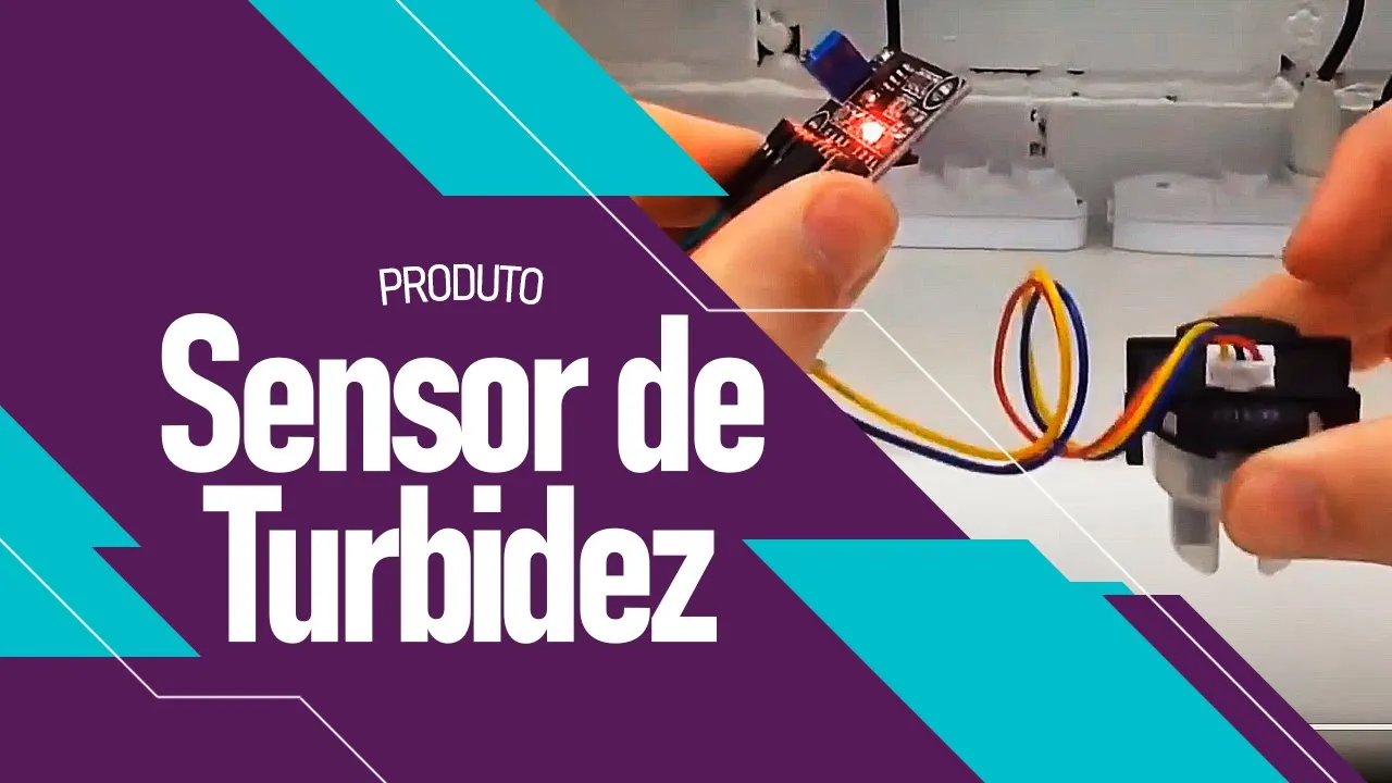
Medindo a Turbidez da Água com Arduino
9.3K
Turbidity measures the light scattering caused by suspended particles in water, expressed in Nephelometric Turbidity Units (NTU), and can be measured using an Arduino with a turbidity sensor that converts voltage readings into NTU values through a quadratic equation (NTU = -120.4 × V² + 574.2 × V - 4352.9), where higher voltage readings indicate greater turbidity.
Click to watch →

STM32 Water Quality Monitor | TDS + Turbidity Sensor with LCD Display
447
Calibration uses the linear equation NTU = m × ADC + b. Measure ADC values at two known conditions: clean water (high ADC, low NTU) and turbid water (low ADC, high NTU). Calculate slope m = (NTU_turbid - NTU_clean) / (ADC_clean - ADC_turbid), then intercept b = -m × ADC_clean. Apply this formula to convert measured ADC values to NTU. Limit results to prevent unrealistic values outside expected range.
Click to watch →

Evaluación de parámetros fisicoquimicos en agua
22.2K
Turbidity measures water clarity using nephelometric units (NTU). The procedure requires calibration with three standard solutions: 0.02 NTU, 1 NTU, and 10 NTU. Steps include: (1) turning on the turbidimeter; (2) accessing the calibration mode using the calibration button; (3) inserting the 1 NTU standard first; (4) waiting for the reading; (5) proceeding to the 10 NTU standard; (6) finally calibrating with the 0.02 NTU standard. After calibration, fill a small container with the sample, ensure the container is clean to prevent interference, place a black cap to block light, insert into the instrument, and press the measurement button. The instrument calculates and displays the turbidity value in NTU.
Click to watch →

수질분석 13 탁도의 정의, 탁도의 단위, 탁도계
1.8K
The Nephelometric Turbidity Unit (NTU) is the modern standard for turbidity measurement, replacing JTU. Unlike JTU which measures transmitted light, NTU measures only scattered light using a sensor positioned at right angles to the light path. This right-angle placement ensures only scattered light enters the detector, avoiding transmitted light interference. NTU is more sensitive for low turbidity measurements because it detects even small amounts of scattered light. However, at high turbidity levels, self-shading occurs - particles in front block light from reaching particles behind, reducing measured scattered light and causing errors. This requires sample dilution for accurate high-turbidity measurements. Different substances interact differently: dark substances like ink absorb light strongly but scatter little, while light-colored substances like chalk powder scatter more than they absorb.
Click to watch →
UPPSC 2024 Ghatna Chakra Purvavlokan Science सम्पूर्ण घटना चक्र पूर्वावलोकन व्याख्यात्मक हल N.K sir
65.3K
Turbidity (जल की विरलता) is measured in Nephelometric Turbidity Units (NTU). This unit measures the cloudiness or haziness of a fluid caused by suspended particles. NTU is commonly used in water quality testing to assess the clarity of water samples. The higher the NTU value, the more turbid the water.
Click to watch →
Deep Dive
Implementing digital signal processing techniques, such as moving average or Kalman filters, to reduce sensor noise in turbulent water.

Filtrage Numérique avec TIA Portal S7-1200 / 1500 - Moyenne mobile, équation de récurrence
5.7K
Digital filtering eliminates noise from sensor signals or smooths trends. Moving average calculates input averages over time intervals: fixed averages compute results after collecting N points, while dynamic averages recalculate at each sample by including new and excluding oldest points. A key trade-off exists: more points improve smoothing but increase delay. Memory requirements grow with window size, potentially causing resource issues.
Click to watch →

C++ & Arduino Tutorial - Implement a Kalman Filter - For Beginners
76.4K
A Kalman filter is an algorithm that provides optimal sensor readings by combining noisy measurements with a mathematical model of the system, using probability theory concepts like mean, covariance, and normal distribution; the filter works by iteratively calculating the Kalman gain to optimally weigh the predicted state against the noisy measurement, with the gain determining the balance between noise reduction and filter responsiveness, and can be implemented in C++ using static variables to maintain state between function calls and adapted for Arduino platforms for real-time sensor noise filtering.
Click to watch →

Probabilistic ML - 11 - Kalman Filters
2.7K
When the transition matrix A is identity (no state evolution) and process noise Q is scalar, the Kalman filter reduces to an exponential moving average. The steady-state Kalman gain becomes a constant value determined by the ratio of observation noise R to process noise Q. The update equation simplifies to m̂ₜ = m̂ₜ₋₁ + K(yₜ - Hm̂ₜ₋₁), which is identical to the exponential moving average update rule. This reveals that any application of exponential moving averages is fundamentally a Kalman filter operating under these specific assumptions, connecting classical signal processing techniques to modern probabilistic frameworks.
Click to watch →
Procesado Digital de Señal con FPGA
1.2K
A moving average filter smooths noisy sensor readings by averaging multiple recent values. The filter uses a register of 8 elements to store recent sensor measurements. New values are added to the left of the register (shifting out the oldest value). The filtered value is calculated by summing all 8 stored values and dividing by 8. This reduces abrupt peaks and valleys in sensor data, making readings more stable and reliable for subsequent processing.
Click to watch →
평균 이동 필터와 칼만 필터를 이용한 노이즈 필터 구현
1.7K
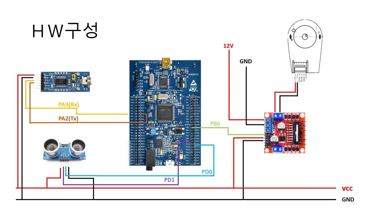
This video explains how moving average filters and Kalman filters can be implemented on STM32F4 boards to reduce noise in ultrasonic sensor distance measurements. The moving average filter calculates the mean of recent data points within a sliding window to smooth out random fluctuations, while the Kalman filter uses probabilistic prediction and correction based on previous estimates and sensor measurements to achieve more accurate results. The Kalman filter demonstrates superior noise rejection compared to the moving average filter, especially for sudden large disturbances, making it more suitable for real-time applications where memory efficiency and computational speed are important considerations.
Click to watch →
Deep Dive
Integrating the turbidity meter into an IoT network (using ESP32 or Wi-Fi shields) for real-time remote environmental monitoring.

Bikin Alat Deteksi Air Keruh Pakai ESP32, Blynk IoT dan Sensor Turbidity! (Tutorial Mudah)
4K
A turbidity sensor measures water clarity by emitting light through the water and detecting scattered light from suspended particles; the more particles present, the more light is scattered, indicating higher turbidity. This tutorial demonstrates building a water quality monitoring system using an ESP32 microcontroller, a turbidity sensor, a voltage divider circuit (10KΩ and 20KΩ resistors) to match the 3.3V ADC input, an LCD I2C display for local visualization, and Blynk IoT for remote monitoring. The system categorizes water quality into three states: clear (0-49), turbid (50-75), and very turbid (76-150), with values displayed on both the LCD and Blynk dashboard.
Click to watch →

cara membuat pompa air otomatis dan sistem monitoring kekeruhan air berbasis IoT turbidity di ESP32
791
This video demonstrates how to build an automatic water pump system with IoT-based turbidity monitoring using ESP32 microcontroller, turbidity sensor, ultrasonic sensor, and relay module, with real-time data transmission to ThingSpeak cloud platform and Android mobile application for remote monitoring and alarm notifications.
Click to watch →

Program sensor turbidity dengan Esp 32
3.5K
This tutorial demonstrates how to integrate a turbidity sensor with an ESP32 microcontroller by installing the Arduino IDE, adding the ESP32 board manager, modifying the ADC reference value from 1023 to 495 for the ESP32, connecting the sensor using color-coded wires (red for VCC, blue for signal, black for GND), and reading the analog values through the Serial Monitor to measure water clarity.
Click to watch →

Sistem Monitoring Kekeruhan Air Secara Realtime Melalui Halaman Website
12K
This video tutorial demonstrates how to build a real-time water turbidity monitoring system using IoT technology, where a NodeMCU ESP8266 microcontroller reads sensor data from a DF Robot turbidity sensor, transmits the values to a PHP web application via HTTP requests, and displays the water quality status (clean, cloudy, or dirty) on a Bootstrap-powered dashboard that updates automatically every second using jQuery's setInterval function.
Click to watch →
MEMBUAT PROJECT ESP32 IOT MONITORING KUALITAS AIR DENGAN SENSOR TDS METER #ESP32 #ESP32PROJECT #iot
10K
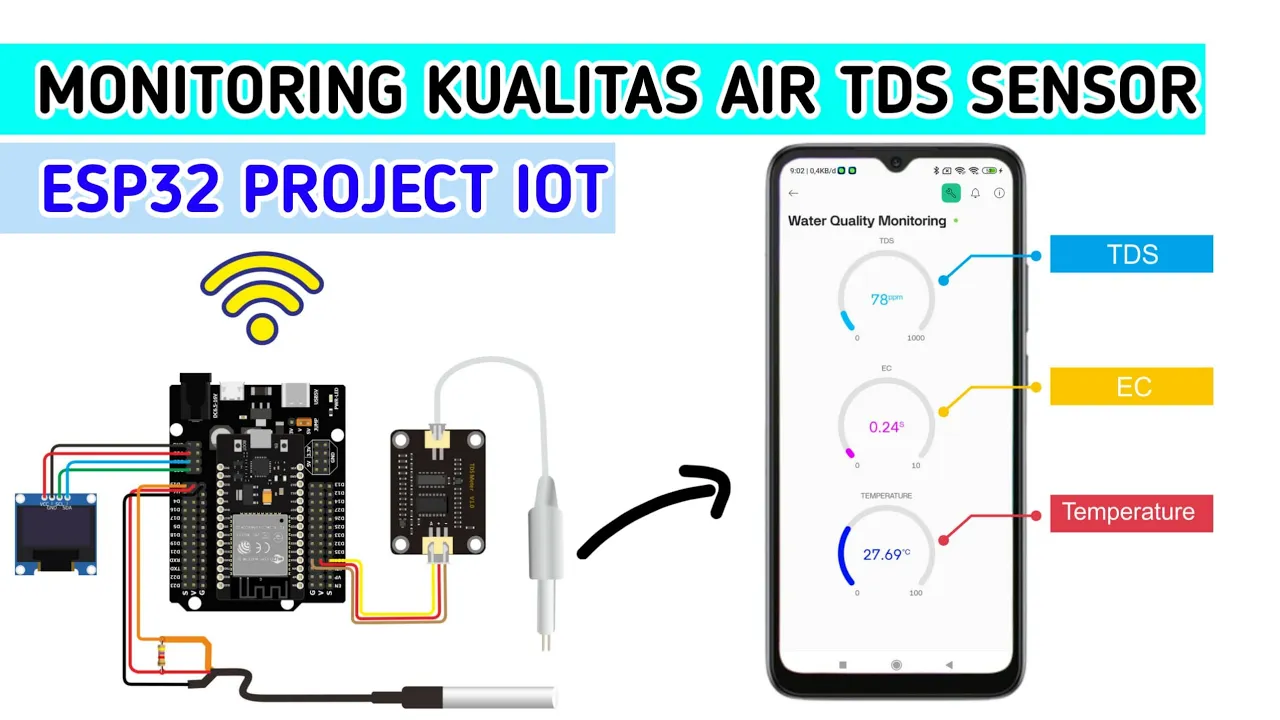
This video demonstrates how to build an IoT water quality monitoring system using ESP32 microcontroller, TDS meter sensor for measuring dissolved solids in PPM and EC units, and DS18B20 waterproof temperature sensor, with real-time data display on OLED LCD and remote monitoring capabilities through Blynk IoT application and Telegram bot.
Click to watch →
Deep Dive
Designing a multi-parameter water quality monitoring station by adding pH, temperature, and electrical conductivity (EC) sensors.

Monitor de PH, temperatura y conductividad electrica de Bluelab
19.7K
The BlueLab Guardian Monitor is a multiparametric device that continuously measures pH, electrical conductivity, and temperature in hydroponic systems, enabling growers to optimize nutrient solution parameters throughout crop growth. Proper setup requires positioning the monitor within 2 meters of the reservoir and 15 meters of power, preparing the pH probe by soaking it in clean water for 1-24 hours before first use, and selecting appropriate measurement units (EC/CF for conductivity, Celsius/Fahrenheit for temperature). Accurate readings depend on regular calibration using pH 7 and either pH 4 or pH 10 solutions, with LED indicators showing calibration status—both LEDs lit indicates valid calibration, while blinking LEDs signal the need for recalibration after 30 days. The device features adjustable alarm thresholds for high and low values across all three parameters, and sensors require periodic cleaning with manufacturer-recommended solutions to maintain measurement accuracy.
Click to watch →

Cool Jobs: GPC's environmental monitoring specialists
127
Water quality monitoring uses multi-parameter sondes that measure pH, dissolved oxygen, electrical conductivity, and temperature. The sensors are cleaned by a wiper mechanism before taking readings to ensure accurate measurements of these key water quality parameters.
Click to watch →

23 June 2023 | A revolution in water quality pH sensing | Mark Pritchard & Richard Campbell
166
The new sensor is a multi-parameter device that simultaneously measures pH, conductivity, and temperature in a single unit. This integration reduces the number of sensors required for water quality monitoring and simplifies deployment. The sensor is designed to be extremely rugged and simple to deploy, transport, and integrate with third-party products and telemetry systems.
Click to watch →

MULTIPARAMETROS PARA AGUA KYNTEL MODELO PH 117
258
Electrical conductivity measures a solution's ability to conduct electricity, which correlates with dissolved nutrient concentration; higher conductivity indicates more dissolved salts and nutrients in the water. In hydroponic cultivation, nutrient solutions typically range from 500-2000 ppm, with safe operating levels around 800-1200 ppm. The PH-117 multi-parameter meter measures pH, temperature, electrical conductivity, and parts per million (PPM), with each parameter requiring separate calibration using standard solutions. Conductivity is measured in microSiemens per centimeter (μS/cm), also known as microOhms per centimeter, and can be converted to PPM or conductivity factor (where 1 conductivity factor equals 0.1 μS/cm).
Click to watch →

11 Mar 22 | Sensor selection for your water quality monitoring application | Ryan Cox
113
Modern water quality monitoring employs multi-parameter probes integrating multiple sensors: standard parameters include pH, dissolved oxygen, and electrical conductivity, with optional ISE and optical sensors covering 95% of applications. Key probe ranges include AP Lite (single parameter), AP 2000 (groundwater applications), and AP 7000 (flagship with six additional ports). Sensor selection requires evaluating measurement range, accuracy (typically 10% of reading), and repeatability. Probes provide qualitative chemistry indications rather than quantitative analysis, requiring lab validation for high-accuracy needs. Most manufacturers design proprietary sensors for better technical support.
Click to watch →
Calibration
Build Meter
Calibration
0:00- 1
Connect sensor to Arduino and measure baseline values.
- 2
Apply blockage to record maximum turbidity reading.
- 3
Store calibrated value for meter configuration.
Limitations of DIY Turbidity Sensors vs. Certified Nephelometric Standards
While building a DIY Arduino-based turbidity meter is an excellent educational exercise, these low-cost consumer sensors have severe limitations compared to professional, certified instrument standards (such as ISO 7027 or EPA Method 180.1). DIY setups typically use simple transmitted light measurement, which is highly sensitive to water color, ambient light, and LED intensity fluctuations. In contrast, regulatory-grade turbidimeters utilize nephelometry—measuring light scattered at a 90-degree angle—and incorporate sophisticated optical filtering, stable light sources, and precise temperature compensation. Without standardized calibration solutions like Formazin, DIY calibration curves are highly prone to drift, making them unreliable for regulatory compliance, scientific research, or critical water safety assessments.
Basic Arduino programming and circuit design, including handling analog and digital I/O pins.
The physical concept of turbidity and how optical sensors measure suspended solids via light scattering (Nephelometry).
Understanding the I2C communication protocol, which is typically used to interface with OLED displays.
Fundamental concepts of sensor calibration, specifically mapping raw analog voltage values to meaningful physical units.
Developing advanced calibration curves using polynomial regression to convert voltage accurately to Nephelometric Turbidity Units (NTU).
Implementing digital signal processing techniques, such as moving average or Kalman filters, to reduce sensor noise in turbulent water.
Integrating the turbidity meter into an IoT network (using ESP32 or Wi-Fi shields) for real-time remote environmental monitoring.
Designing a multi-parameter water quality monitoring station by adding pH, temperature, and electrical conductivity (EC) sensors.
31.6K views369likes3:09@EDISON_SCIENCE_CORNEROriginal Release: 2023-01-08
hello there in this video tutorial I'm going to show you how to build a turbidity meter using turbidity module and Arduino I'm also showing how to calibrate this durability sensor let's get started with this video so here is the turbidity module and the amplifier the amplifier has three pins VCC ground and the output working and other details of this module I explained in a previous video you can find that video from the I button first let's see how to calibrate the sensor for that connect the VCC to 5 volt of Arduino ground to ground and the analog pin to a0 pin of Arduino and that's it now connect the Arduino to computer and open Arduino IDE now go to file examples basics select the analog grade serial code now select the board and port and upload the code after uploading the code open the serial Monitor and you can see the serial data now apply some blocking material in between the sensor just like in the video and not that value that value is the maximum turbidity value also not the dead value now let's build the turbidity meter so I connected the OLED display to the Arduino round to ground VCC to five volt SDA to A4 and ACL to A5 also I conducted a RGB LED you can download the code and circuit diagram from my website link is given in the description here is the code in this line you have to replace this value with your calibrated value and that's it now upload this code and see the working so this is how I made a turbidity meter using Arduino and terability module hope you enjoyed and learned something new from my video if so please like share and subscribe thanks for watching I will see you next time
Up Next
12:00
How to Calibrate an Analog pH Sensor for Arduino and Raspberry Pi
@DavyBot
51.3K views•2018-11-18

12:54
Triumph of Orthodoxy Icon: Byzantine Art & History Explained
@BenCallan
2.1K views•2024-08-06
6:42
Arduino Turbidity Meter: Complete DIY Sensor Tutorial
@EDISON_SCIENCE_CORNER
58.1K views•2020-09-01

1:42
Game of Thrones Opening Credits: A Cinematic Analysis
@gameofthrones
46.3M views•2011-04-18
Related Study Plans & Knowledge Roadmaps
Structured learning paths in General & Interdisciplinary Studies
general-studies
Elevator Engineering: History, Physics & Cities
01From Hoists to Safety Brakes: The Dawn of Vertical Lift
02Hydraulic vs. Traction: The Engineering Physics of Elevators
03Modern Speed, Safety, and Algorithms
+ 2 more learning modules
12h5 modules
Explore Roadmap
general-studies
Rubber: Material Science, History & Geopolitics
01Origins of Natural Rubber & Mesoamerican History
02The Chemistry of Natural Rubber & Vulcanization
03The Geopolitics of the Rubber Boom & Colonization
+ 2 more learning modules
12h5 modules
Explore Roadmap
general-studies
Containerization: Evolution, Logistics & Trade
01Ancient Trade & Bulk Cargo: Amphorae to Barrels
02The Industrial Revolution & Cardboard Packaging
03The Containerization Revolution: Malcom McLean
+ 2 more learning modules
12h5 modules
Explore Roadmap
general-studies
Textile Tech: Evolution, Labor & Global Impact
01Pre-Industrial Textiles: Handloom & Cottage Industry
02Mechanization: The Spinning Jenny to the Power Loom
03The Factory System & Global Labor Transformation
+ 2 more learning modules
10h5 modules
Explore Roadmap