This video tutorial demonstrates how to generate a quantitative PCR (qPCR) standard curve and calculate PCR assay efficiency using Google Sheets. The process involves plotting threshold cycle (Ct) values against known template concentrations to create a linear regression curve, from which PCR efficiency can be calculated using the formula E = 10^(-1/slope) - 1. The instructor guides viewers through importing experimental data, creating scatter plots, adding trendlines, and performing mathematical calculations to determine the amplification efficiency of their qPCR assays.
How to Calculate qPCR Efficiency Using a Standard Curve in Google Sheets
Added:Deep Dive
Basic principles of Real-Time Quantitative PCR (qPCR), including the definition and significance of the cycle threshold (Ct or Cq) value.

RT - PCR (Real Time PCR) | Quantitative - PCR | qPCR | Basic Principle and Data Analysis
131.7K
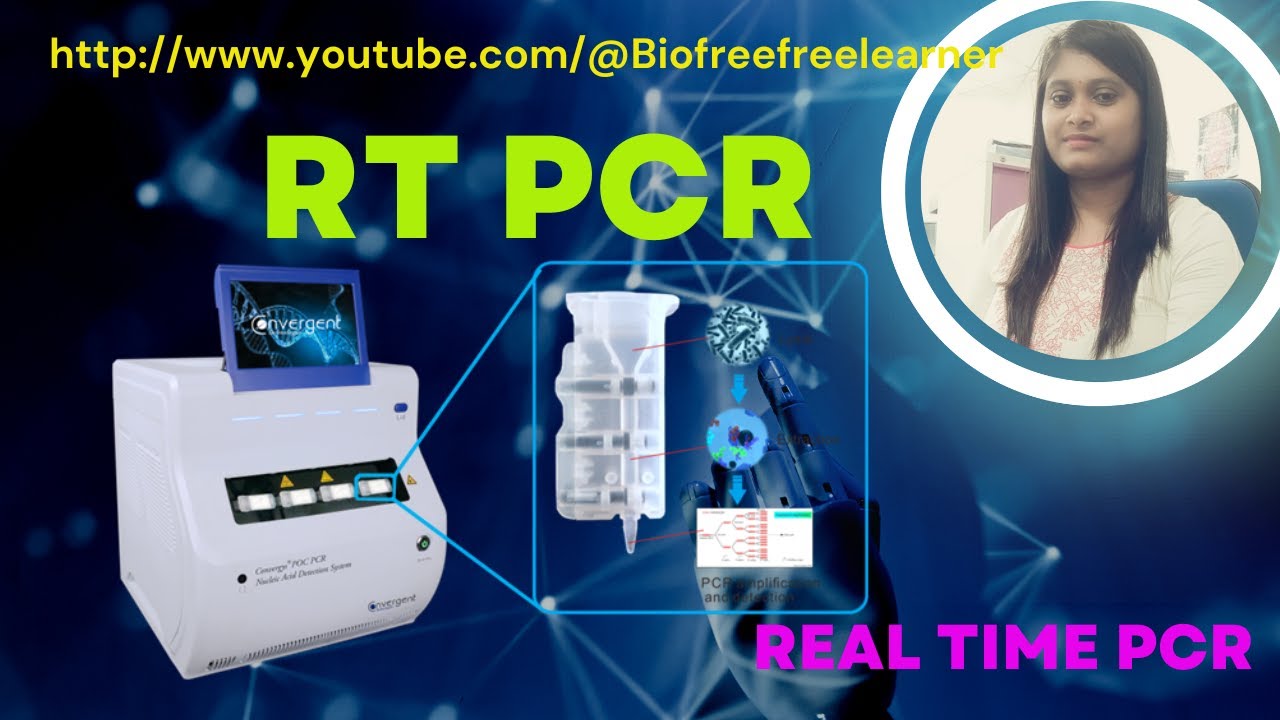
Real-Time PCR (quantitative PCR or qPCR) is a molecular biology technique that amplifies and simultaneously quantifies DNA or RNA in real-time by monitoring fluorescence signals during the amplification process. Unlike traditional PCR which provides endpoint measurements, qPCR uses fluorescent dyes (like SYBR Green) or sequence-specific probes to detect amplified products continuously. The technique involves three main steps: denaturation (95°C), annealing (57-60°C), and extension (72°C), with Taq polymerase synthesizing new DNA strands. During extension, if probes are used, the enzyme's 5' to 3' exonuclease activity cleaves the probe, separating the fluorescent reporter from the quencher and generating a measurable signal. The amplification curve generated shows fluorescence intensity versus PCR cycle number, and the threshold cycle (Cq) value—the point where the signal crosses above background—is inversely proportional to the initial template concentration. Lower Cq values indicate higher initial DNA/RNA amounts, enabling precise quantification of genetic material for applications like viral load detection.
Click to watch →
Quantitative PCR | QPCR | Real Time PCR
610
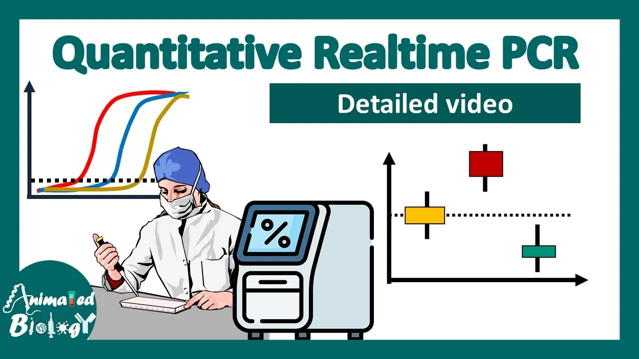
Quantitative PCR (qPCR) is a real-time PCR technique that monitors DNA amplification during the reaction using fluorescent reporters, allowing researchers to quantify the initial amount of nucleic acid template by measuring the cycle threshold (Ct) value, where lower Ct values indicate higher template concentrations; the technique employs either SYBR Green dye or probe-based methods for detection and requires proper controls including negative controls to ensure accurate results.
Click to watch →

What is PCR and qPCR? | PCR Animation
252.9K
PCR (Polymerase Chain Reaction) is a revolutionary molecular biology technique invented by Kary Mullis in 1983 that enables unlimited DNA amplification through repeated cycles of heating (95°C to separate DNA strands), cooling (60°C for primer binding), and DNA synthesis by Taq polymerase; qPCR (quantitative PCR) extends this by adding fluorescent probes that emit light when cleaved during amplification, allowing real-time monitoring and quantification of DNA through the cycle threshold (Ct) value, which correlates with initial DNA quantity (a 2-cycle difference equals 4 times more DNA, 20 cycles equals 1 million times more), enabling applications from disease diagnosis to multiplex detection of multiple pathogens in single tests.
Click to watch →
Quantitative Real-Time PCR (qPCR): Principle, Method & Data Analysis
129.2K
Quantitative real-time PCR (qPCR) is a molecular biology technique used to detect and quantify specific RNA molecules in real-time during amplification. The method relies on SYBR Green dye, which fluoresces only when bound to double-stranded DNA, allowing the machine to monitor DNA accumulation cycle-by-cycle. The cycle threshold (CT) value indicates the amplification point where fluorescence crosses a detection threshold, with lower CT values signifying higher initial template abundance. Data analysis uses the ΔΔCT method for relative quantification, comparing target gene expression against reference genes. Melt curve analysis verifies amplification specificity by monitoring fluorescence as temperature increases, ensuring only the desired product was amplified. Successful qPCR requires optimal reaction conditions, proper primer design, high-quality RNA/cDNA templates, and careful pipetting techniques.
Click to watch →

Understanding real-time PCR terminology--Taq Talk Episode 1
32.2K
Real-time PCR (quantitative PCR or qPCR) is a technique that detects fluorescent signals during each PCR cycle to quantify target nucleic acids; key terminology includes RT for reverse transcription (converting RNA to cDNA), Cq (quantification cycle) which indicates the cycle number when amplification crosses the threshold above baseline fluorescence (with lower Cq values indicating higher target expression), and analysis methods like delta CT (difference between target and control gene CT values) and delta-delta CT (comparing normalized delta CT values between samples).
Click to watch →
Deep Dive
The concept of serial dilutions and how to calculate dilution factors to prepare standard curve samples.

8. Curva de calibración | Análisis Instrumental
85.7K
To prepare multiple standards from a mother solution, serial dilutions are performed using aliquots transferred to volumetric flasks. For example, starting with a mother solution of 1.213 mg/mL: taking 2 mL and diluting to 50 mL gives 0.049 mg/mL; taking 4 mL and diluting to 50 mL gives 0.097 mg/mL; taking 6 mL gives 0.146 mg/mL; taking 8 mL gives 0.194 mg/mL; taking 10 mL gives 0.243 mg/mL; and taking 12 mL gives 0.291 mg/mL. This creates six standards with progressively increasing concentrations for the calibration curve.
Click to watch →
Serial dilution calculations | How to calculate dilution factor - Dr K
92.2K
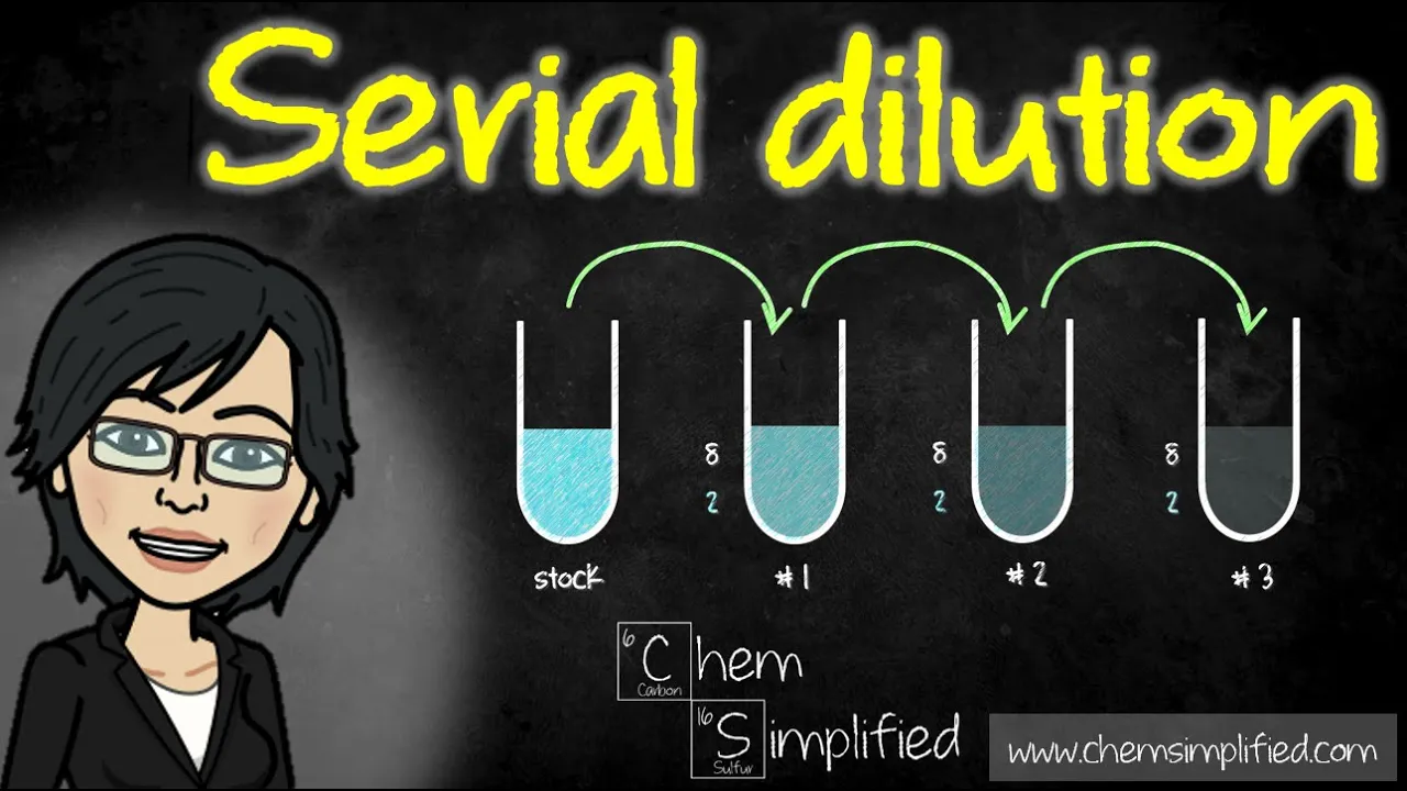
Serial dilution is a laboratory technique where a solution is diluted in a series of steps, with each step reducing the concentration by a specific factor; the dilution factor for each step is calculated as the ratio of the volume of stock solution to the total volume of the diluted solution, and the total dilution factor across multiple steps is found by multiplying the individual dilution factors together. For example, three rounds of 5-fold serial dilution result in a total dilution factor of 125-fold (5 × 5 × 5), making it possible to work with very concentrated solutions by progressively reducing their concentration to measurable levels.
Click to watch →

Serial dilutions and pour plate technique
337.1K
Serial dilution is a fundamental microbiological technique for quantifying bacteria in unknown samples. The process involves creating progressively more dilute solutions by transferring measured amounts of sample to volumes of sterile water. A 1:10 dilution (1 mL sample + 9 mL water) equals 0.1 or 10^-1. For solid samples, 1 gram is equivalent to 1 mL liquid. Total dilution in each tube is calculated by multiplying individual transfer dilutions together, adding exponents when bases are the same. Alternative schemes use 99 mL bottles for 10^-2 dilutions. Single dilution calculations consider only the current transfer, while total dilution accounts for cumulative dilution from all previous steps.
Click to watch →

How to prepare a Serial Dilution
337.1K
A serial dilution is a stepwise dilution by a constant factor (typically 10-fold or 2-fold) where each subsequent dilution step contains progressively less of the original solution; for a 10-fold dilution, you fill tubes to 9/10 of their capacity, add 1 part of the stock solution to create a 1:10 dilution, then transfer 1 part of each diluted solution to the next tube with fresh diluent to achieve 1:100, 1:1000, and so on, while for a 2-fold dilution, you mix equal volumes of stock and diluent at each step.
Click to watch →
Dilution and Dilution Factor in Microbiology|| How to Calculate Dilution factor in Serial dilution?
62.9K
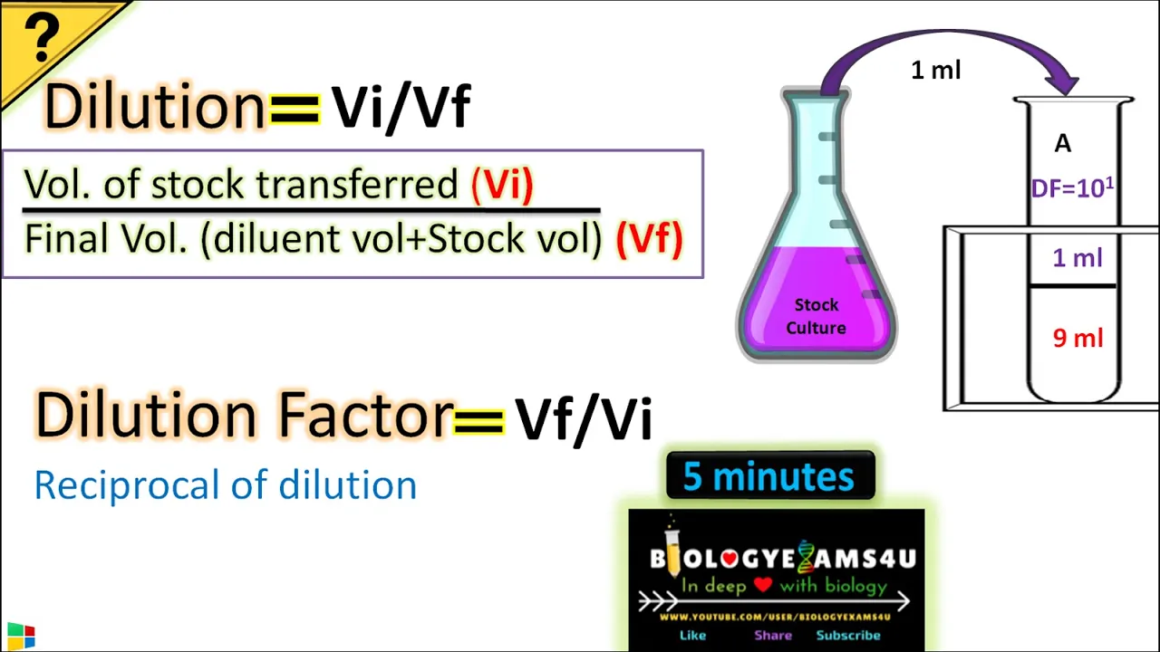
In microbiology, dilution is calculated as the ratio of initial volume (Vi) to final volume (Vf), while dilution factor is its reciprocal (Vf/Vi); for example, transferring 1ml stock into 9ml diluent creates a 1/10 dilution with a dilution factor of 10:1, and in serial dilution, the total dilution factor is obtained by multiplying the dilution factors of each successive step (e.g., four steps of 10:1 each yield a total dilution factor of 10,000).
Click to watch →
Deep Dive
Fundamental spreadsheet skills in Google Sheets, including data entry, applying basic formulas, and plotting scatter graphs.

Working Scientifically - Part 3 - Results, Tables and Graphs
474
To create a scatter graph in Google Sheets, copy your data including labels and units, go to the Chart menu, select XY scatter plot, adjust the y-axis to start at zero, add axis labels with units, insert a line of best fit (linear), and optionally display the R-squared value to show correlation strength between variables.
Click to watch →

2강_데이터 입력
5K
Google Sheets supports numbers (right-aligned, supports percentages and thousands separators), text (left-aligned, force with single quote), dates (use hyphens or slashes), and times (use colons). Ctrl+Enter serves dual purposes: creating line breaks and filling selected ranges. The Input Tool (Ctrl+Shift+K) provides alternative entry. Formulas begin with = and Google Sheets provides automatic suggestions. Basic operators include +, -, *, /, and ^. The plus key substitutes for equals. Edit cells by double-clicking or pressing F2. Delete clears content while right-click delete can shift cells.
Click to watch →
MÓDULO 12 Semana 3 ► Actividad integradora 5 y 6 👌
32K
To create graphs in Google Sheets: (1) Enter data in columns, (2) Select the data range, (3) Go to Insert > Chart, (4) Choose the appropriate chart type (scatter plot for energy vs. time), (5) Customize labels and axes. The spreadsheet automatically calculates values using formulas.
Click to watch →

C.1 Lesson 10 Simulation Data Analysis | Scatter Plots in Google Sheets
433
To create a scatter plot in Google Sheets, first select the data columns you want to graph (mass times change in temperature for the X-axis and change in energy for the Y-axis). Go to Insert and select Chart. If Google Sheets doesn't give you the desired chart type, click on an empty cell and insert a chart from scratch. Select 'Scatter Plot' as the chart type. Then specify your data range, which tells Google Sheets which column goes on the X-axis and which on the Y-axis.
Click to watch →

Google Sheets Telugu Tutorials | 02 | Telugu, Hindi Data Entry, Formulas, Format Options | Beginners
126.6K
This segment covers the foundational aspects of Google Sheets data entry, including understanding different data types, entering information into spreadsheets, and managing basic spreadsheet operations. The content emphasizes the importance of proper data entry techniques for accurate record-keeping and data management.
Click to watch →
Deep Dive
The mathematical theory of linear regression, specifically understanding slope, y-intercept, and the coefficient of determination (R²).
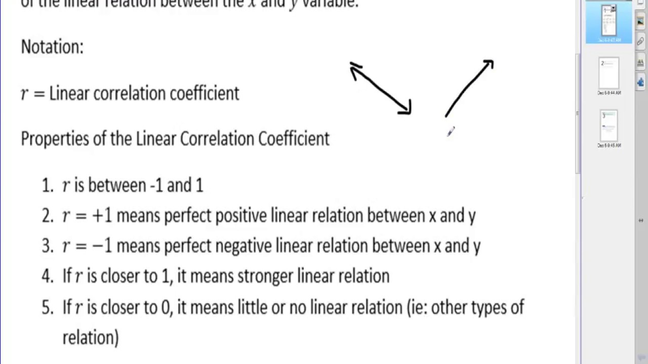
120 12.1-12.2
155
The slope (b) indicates the change in Y for each unit increase in X. A negative slope indicates negative linear correlation (as X increases, Y decreases). The y-intercept (a) represents the predicted Y when X = 0. When X = 0 in the regression equation, the predicted value equals the y-intercept. The coefficient of determination (R²) indicates model fit quality. For example, R² = 0.778 means approximately 78% of Y's variation is explained by X.
Click to watch →

p03 regresion
260
Linear regression creates mathematical models that approximate relationships between variables by finding the best-fit line that minimizes error. The slope represents the rate of change: for every one-unit increase in the independent variable, the dependent variable changes by the slope amount. The intercept is the starting value when x equals zero. The sign of the slope indicates relationship direction: positive for direct relationships, negative for inverse relationships. The coefficient of determination (R²) measures model quality, ranging from 0 to 1. Values near 1 indicate good fit, while values near 0 indicate poor fit. Before regression analysis, prepare data by loading datasets into statistical software. Correlation analysis examines relationships between multiple variables simultaneously through a correlation matrix.
Click to watch →

Interpretations for r, r-squared, slope, intercept
2.7K
In regression analysis, the slope represents the change in the predicted dependent variable (Y) for each one-unit increase in the independent variable (X), the intercept represents the predicted Y value when X equals zero, the correlation coefficient (R) indicates the strength and direction of the linear relationship (ranging from -1 to +1), and R² represents the percentage of variance in Y that is explained by X.
Click to watch →

OpenStax Statistics Ch 12.1,3 and 5 Regression equation # 1
756
Linear regression is a statistical method that finds the best-fit line (y = a + bx) to predict a dependent variable (Y) from an independent variable (X), where 'a' is the y-intercept and 'b' is the slope representing the rate of change; the coefficient of determination (R²) measures how well the line fits the data by showing the proportion of variation in Y explained by X.
Click to watch →

StatLecture Ch12 Linear Regression Equation Part 2
139
In linear regression, the slope represents the rate of change in the dependent variable (Y) for each unit increase in the independent variable (X), while the y-intercept represents the predicted value of Y when X equals zero; both must be interpreted in the context of the specific problem, and the coefficient of determination (R²) measures the proportion of variation in Y explained by the regression model, indicating how well the model fits the data.
Click to watch →
Prerequisite Knowledge
- Concept 01Basic principles of Real-Time Quantitative PCR (qPCR), including the definition and significance of the cycle threshold (Ct or Cq) value.
- Concept 02The concept of serial dilutions and how to calculate dilution factors to prepare standard curve samples.
- Concept 03Fundamental spreadsheet skills in Google Sheets, including data entry, applying basic formulas, and plotting scatter graphs.
- Concept 04The mathematical theory of linear regression, specifically understanding slope, y-intercept, and the coefficient of determination (R²).
Subsequent Learning
- Step 01Applying the calculated assay efficiency to relative gene expression calculations using the Pfaffl method.
- Step 02Troubleshooting qPCR assays when efficiency falls outside the ideal 90–110% range, such as identifying pipetting errors or PCR inhibitors.
- Step 03Designing and validating multiplex qPCR assays where multiple target genes are quantified in a single reaction.
- Step 04Transitioning data analysis to advanced bioinformatic tools or programming languages like R for high-throughput qPCR workflows.
Opening Notes
Rhythm Build
Core Melody
Audience Peak
Mood Shift
Vocal Entry
Dynamic Swell
Final Crescendo
Closing Notes
Opening Notes
0:41Playing Section
- 1
Musical introduction sets the initial tone.
- 2
Applause marks the beginning of the session.
Individual Curve-Fit Kinetic Analysis
While the standard curve method is widely used to calculate qPCR efficiency, it relies on the flawed assumption that efficiency is constant across all dilution levels and biological samples, ignoring potential matrix effects, pipetting errors, or sample-specific inhibitors. An alternative approach is individual curve-fit kinetic analysis (such as the Cy0 method or sigmoidal curve fitting). This methodology estimates amplification efficiency directly from the fluorescence data of each individual reaction's amplification curve, rather than relying on an external dilution series. This allows for sample-specific efficiency assessment, saves reagents and template DNA, and avoids the propagation of dilution errors. Furthermore, critics argue that performing these complex mathematical calculations in spreadsheet software like Google Sheets is error-prone and lacks the reproducibility offered by dedicated programming packages (such as R's 'qpcR') or specialized qPCR analysis software.
Deep Dive
Applying the calculated assay efficiency to relative gene expression calculations using the Pfaffl method.
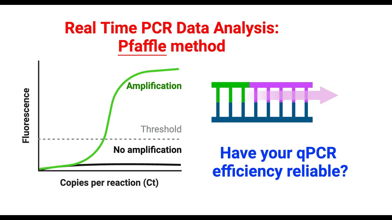
Real Time PCR data analysis using Pfaffle method | step-by-step tutorial |
493
The Pfaffl method is a quantitative PCR data analysis technique used to calculate relative gene expression levels by accounting for PCR amplification efficiency, which is particularly useful when PCR efficiency is close to the ideal value of 2.0; the method involves calculating the average threshold cycle (Ct) values for both the target gene and reference gene across control and treated samples, determining the difference in Ct values (ΔCt), applying the mean PCR efficiency to this difference using the formula E^(-ΔCt), and finally calculating the fold change by dividing the efficiency-corrected values of the target gene between experimental conditions.
Click to watch →

Real Time QPCR Data Analysis Tutorial (part 2)
300.9K
This tutorial explains three primary methods for analyzing real-time quantitative PCR data: the Livak method (delta delta CT), which normalizes target gene expression against a reference gene and then against a calibrator sample to calculate fold change; the delta CT method, which calculates relative expression values for each sample and divides by the calibrator's expression value; and the Pfaffl method, which accounts for differences in amplification efficiencies between target and reference genes using their respective efficiencies in the calculation. The choice of method depends on whether reaction efficiencies are similar (Livak/delta CT) or different (Pfaffl), with all methods relying on CT values for quantification.
Click to watch →

Validating differential gene expression: Methods, Sarah Diermeier, Ph.D.
11.2K
The delta-delta CT method calculates relative gene expression: ΔCT = CT(target) - CT(control) for both calibrator and experimental samples; ΔΔCT = ΔCT(experimental) - ΔCT(calibrator); RQ = 2^(-ΔΔCT). This assumes equal primer efficiencies between target and control genes. Efficiency should be measured by plotting ΔCT vs log(relative quantity); ideal slope = -3.32 (100% efficiency), acceptable range = 95-105%. If efficiency falls outside this range, new primers should be designed or efficiency-corrected calculations applied. Efficiency-corrected formula: RQ = E^(-ΔΔCT), where E is primer efficiency. Always run multiple primer pairs per target and verify results with gel electrophoresis and melting curves.
Click to watch →

Real Time QPCR Data Analysis Tutorial
630K
Real-time quantitative PCR detects amplicon accumulation in real-time, generating threshold cycle (CT) values that correlate inversely with starting template amount; absolute quantification determines exact nucleic acid quantities using standard curves and linear regression equations, while relative quantification compares gene expression changes between samples using normalization methods such as delta CT (Livak method) or Pfaffl method accounting for amplification efficiency differences.
Click to watch →

How real-time PCR assay efficiency can affect your data--Taq Talk Episode 32
1.8K
Real-time PCR assay efficiency, ideally 100% (meaning template doubles exactly every cycle), significantly impacts data accuracy; for reliable relative quantification using the delta-delta CT method, target and reference assay efficiencies must be within 10% of each other, and deviations from 100% efficiency—whether due to inhibitors causing apparent efficiencies over 100% or suboptimal reaction conditions causing efficiencies under 100%—can reduce calculation accuracy, requiring validation through dilution series and standard curve analysis with R-squared values above 0.99.
Click to watch →
Deep Dive
Troubleshooting qPCR assays when efficiency falls outside the ideal 90–110% range, such as identifying pipetting errors or PCR inhibitors.

Resolving Poor PCR assay Efficiency in Real Time PCR
1.9K
Real-time PCR assay efficiency, defined as the rate at which target DNA is amplified during each thermal cycle, is a critical quality metric for quantitative PCR assays; an ideal efficiency of 100% (corresponding to a standard curve slope of -3.32) indicates optimal assay performance, while values outside the acceptable range of 90-105% suggest either inhibition (efficiency >105%) or poor reaction conditions (efficiency <90%), requiring troubleshooting through template dilution, re-purification, buffer optimization, primer/probe adjustment, and thermal cycling parameter refinement to achieve reliable quantification.
Click to watch →

Webinar Fundamentos de PCR Tiempo Real
129
Poor primer design causes 99% of PCR failures, not kit or machine issues. When reactions fail, increase annealing temperature (60°C to 62-65°C) and reduce annealing time (<15 seconds). Increasing template amount (1-2 μL to 5-6 μL) can improve results, but maximum template load is 200 nanograms. Diluting cDNA (1:10) and using larger volumes improves sample representation. PCR efficiency should exceed 90% (ideally 95%) for accurate quantification, calculated from standard curves using serial dilutions. Common inhibitors include polyphenols/humic acids from soil, residual alcohol from extraction, and pH changes in water.
Click to watch →
![[Recording] Webinar: qPCR 101](https://i.ytimg.com/vi/2aUt9AEArzQ/maxresdefault.jpg)
[Recording] Webinar: qPCR 101
972
This section covers qPCR chemistry selection and assay optimization. Two main chemistries exist: SYBR Green (intercalating dye) offers sensitivity and low cost but requires specificity verification via melt curves and gels; hydrolysis probes (TaqMan) provide high specificity and multiplexing capability (2-5 targets) but higher cost. Assay design requires: 70-200 bp amplicons, 50-60% GC content, intron-spanning primers for gene expression, similar annealing temperatures (~60°C), and avoidance of GC clamps, secondary structures, and primer-dimers. Probe-based assays require probes 5-10°C higher than primers with 30-80% GC content. Validation requires: sequence validation using OligoEvaluator, optimization of primer/probe concentrations and annealing temperature via gradient PCR, standard curve validation (10-fold dilutions in triplicates), and melt curve analysis. Acceptable efficiency is 90-110%. Essential controls include water negative control, positive control, and no-RT control. Reference genes must be validated for stability in specific conditions, with at least two genes recommended. Troubleshooting poor signal involves checking positive control first, then sample quality or assay optimization. Poor reproducibility requires pipette calibration, larger volumes, primer-dimer checks, and potential assay redesign.
Click to watch →
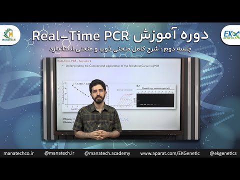
آموزش کامل Real-Time PCR - جلسه دوم : شرح کامل منحنی ذوب و منحنی استاندارد
673
The R² value indicates how well standard curve data fits the linear model, with values close to 1 indicating accurate serial dilutions. Acceptable PCR efficiency ranges from 90-110%, with 100% being ideal. Efficiency below 90% indicates suboptimal reaction conditions, while efficiency above 100% typically indicates the presence of inhibitors in the sample. PCR inhibitors (hemoglobin, heparin, extraction reagents) interfere with DNA polymerase activity and primer binding, reducing reaction efficiency. Inhibitors cause apparent efficiency above 100% because they delay amplification in high-concentration samples but have less effect in diluted samples. This creates a steeper slope (less negative) in the standard curve. The slope becomes less negative (e.g., -0.8 instead of -1), resulting in calculated efficiency above 100%. Proper sample preparation and dilution can minimize inhibitor effects.
Click to watch →

Discover Real-Time PCR for the Classroom
57.3K
Successful real-time PCR requires careful optimization and systematic troubleshooting. Well-optimized reactions show evenly spaced points on standard curves with replicates perfectly overlapping—tenfold serial dilutions should be approximately 3.3 CT units apart at 100% efficiency. Optimization involves empirically testing multiple primer sets and performing temperature gradient runs to find optimal annealing conditions. Common troubleshooting issues include non-flat baselines (pipetting errors, evaporation, bubbles), poorly clustered replicates (pipetting inconsistency, optimization problems), improperly spaced dilution series (pipetting errors, PCR inhibitors, insufficient DNA), and non-sigmoid curves (evaporation, assay problems, electrical noise). Real-time PCR provides excellent opportunities to teach experimental design principles, as analyzing problematic data reveals how factors like pipetting technique, plasticware choice, plate sealing, and proper control use affect results. This transforms troubleshooting into valuable learning experiences about scientific methodology and reproducibility.
Click to watch →
Deep Dive
Designing and validating multiplex qPCR assays where multiple target genes are quantified in a single reaction.

MIQE Guidelines: A Roadmap for Proper qPCR Experimental Design and Reporting
12.8K
Multiplex qPCR (amplifying multiple targets in a single reaction) presents significant challenges. Practical experience indicates that successfully amplifying four targets simultaneously is difficult, and achieving five working targets is rare. Best practices: (1) Only pursue multiplexing when substantial cost savings justify the effort, such as in diagnostic applications where the same assay is repeated many times. (2) Test different commercial kits that claim to improve multiplexing performance. (3) Ensure individual assays work well separately before attempting multiplexing. (4) Monitor amplification efficiencies of each target when combined, as efficiencies may change when assays are mixed together. The trade-off between reagent savings and increased complexity must be carefully weighed.
Click to watch →
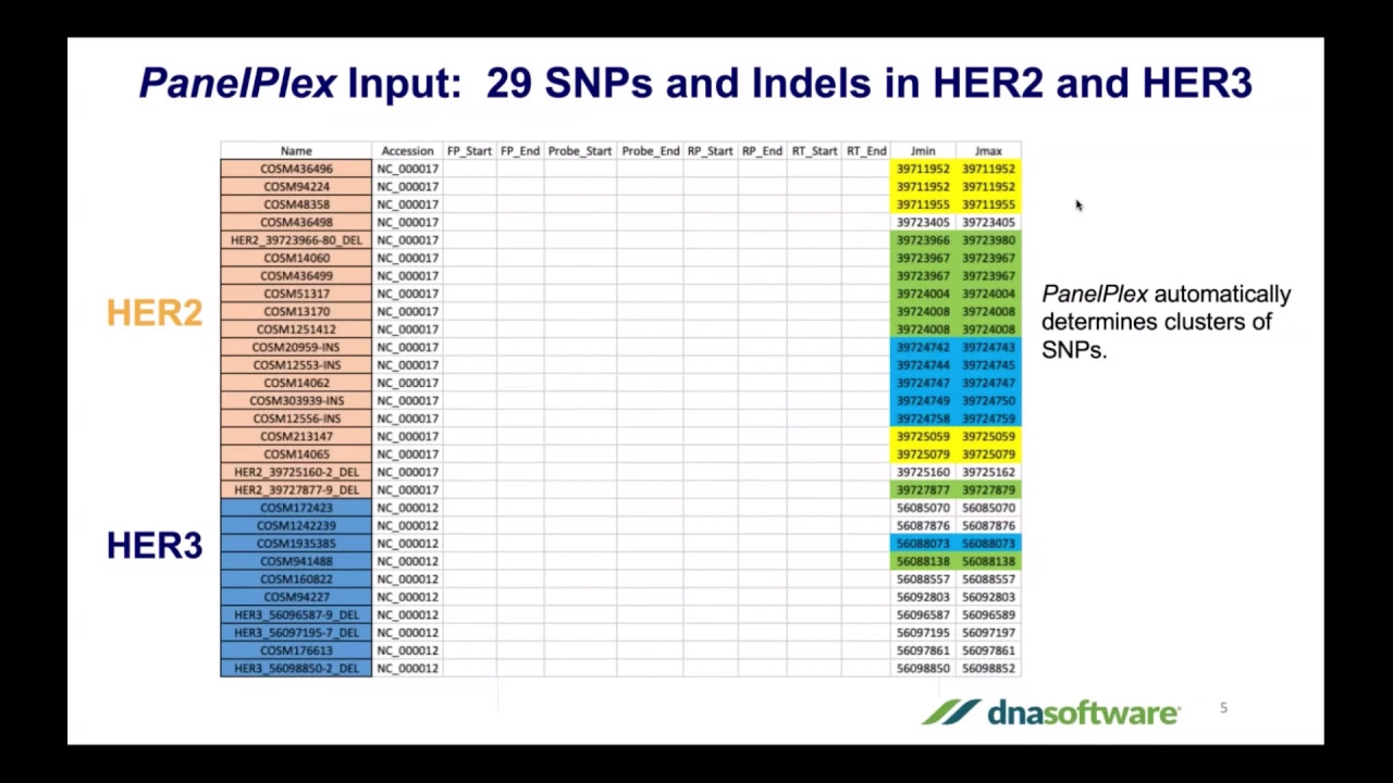
PanelPlex Demo (Multiplex PCR assay design software)
728
Effective multiplex PCR assay design requires understanding how to manage multiple genetic targets within a single reaction. The software handles SNP clustering by automatically combining targets that are too close together (typically within 3-42 nucleotides) to have separate amplicons. Users select between multiplex mode (designing compatible primers for simultaneous detection) and batch mode (creating separate assays for each target). Key settings include gap parameters controlling amplicon size (minimum 25 nucleotides between primers, maximum determining total amplicon length around 140 nucleotides). The system intelligently groups mutations, insertions, deletions, and SNPs into combined assays, reducing the total number of required reactions while maintaining detection capability.
Click to watch →
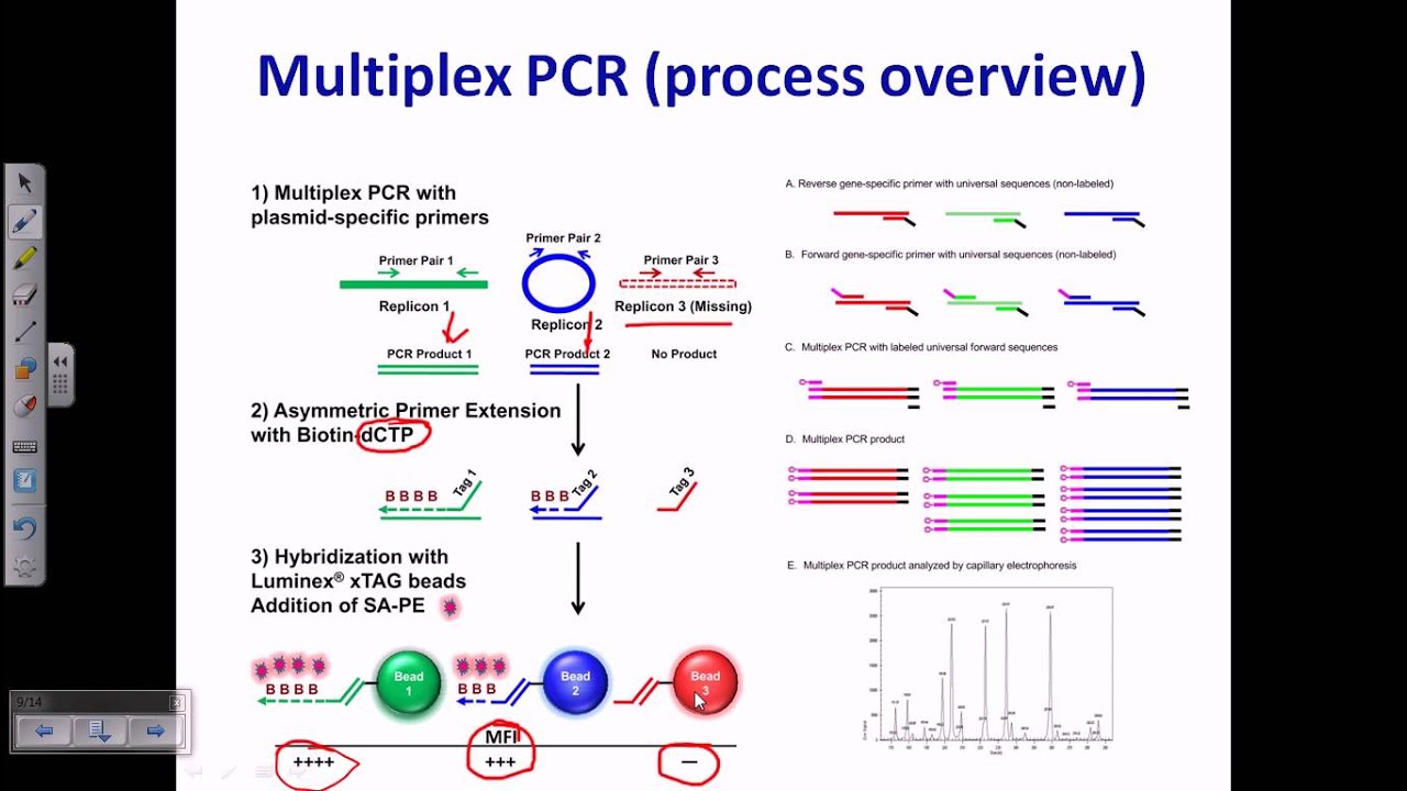
PCR types
221.1K
Multiplex PCR allows simultaneous amplification of multiple target sequences in a single reaction tube using multiple primer pairs. This technique saves time and resources compared to running separate PCRs for each target. However, careful primer design is essential to prevent cross-hybridization between primers and templates. Applications include detecting the presence and relative abundance of different replicons or genes within a sample, with quantitative analysis possible through tagging strategies like biotin-labeled dCTP and detection via luminescent dyes.
Click to watch →

Multiplex RT-qPCR: Advanced Gene Expression Analysis with PrimePCR Assays
674
Multiplex RT-qPCR enables simultaneous detection and quantification of multiple RNA targets in a single reaction by combining reverse transcription with quantitative PCR, offering cost-effective gene expression analysis through reduced pipetting and increased throughput; successful assay design requires upfront optimization including selecting primers/probes with minimal homology, using fluorophores with minimal spectral overlap to minimize cross-talk, testing each assay's dynamic range and efficiency in singleplex before multiplexing, and ensuring PCR efficiencies remain consistent when combining assays.
Click to watch →
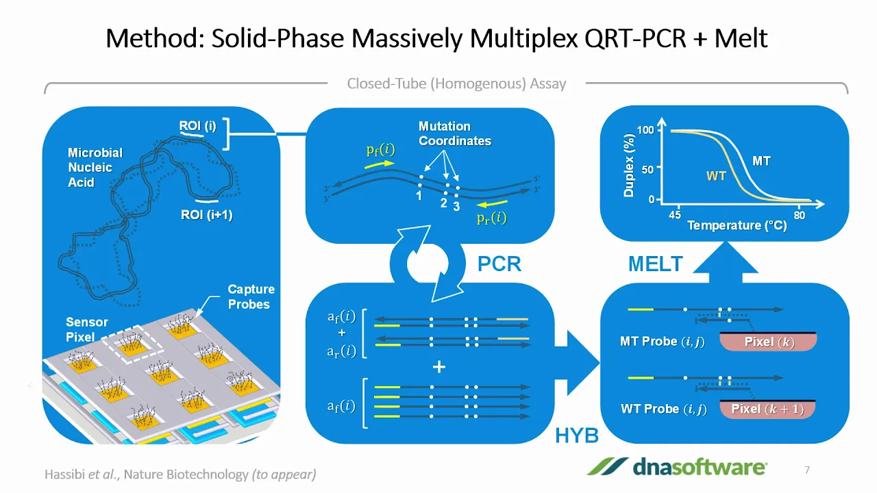
Multiplex PCR Assay Design Made Easy
7.3K
The Hydra platform implements solid phase multiplex quantitative RT-PCR using CMOS biochips in disposable cartridges, enabling up to 1024 targets simultaneously. The technology involves asymmetric PCR creating single-stranded amplicons captured by surface probes, followed by solid-phase melt analysis for sequence differentiation. A comprehensive assay development pipeline includes: (1) specification and requirements setup with inclusivity/exclusivity criteria and GenBank database building; (2) bioinformatics processing with automated primer design, rigorous computational review, and probe design; (3) experimental qualification including singleplex screening, ranking, down-selection, characterization, guard band testing, and multiplex debugging. This systematic approach, combined with automated design tools, enabled development of a comprehensive upper respiratory panel with 27 viruses and 3 bacterial targets in approximately four months with minimal personnel.
Click to watch →
Deep Dive
Transitioning data analysis to advanced bioinformatic tools or programming languages like R for high-throughput qPCR workflows.
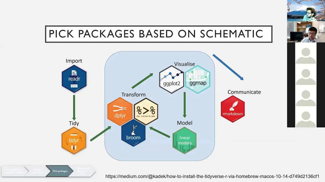
R for Biologists (Week #5)
5.1K
This lesson demonstrates how to use the tidyverse package in R to analyze qPCR data through a systematic workflow: reading tab-delimited data files, cleaning data by selecting relevant columns, removing NA values and undetermined entries, converting data types to numeric, calculating delta CT values by subtracting housekeeping gene CT values from target gene CT values, computing average delta CT and standard deviation across replicates, and visualizing results using ggplot2 with error bars. The key tidyverse verbs used include read_delim(), select(), drop_na(), filter(), mutate_at(), group_by(), summarize(), and join().
Click to watch →

One click qPCR script in R.
1.2K
This video demonstrates an R script that automates qPCR data analysis by loading metadata from Excel files, calculating relative gene expression using the delta-delta Ct method (which compares target gene expression to housekeeping genes across different experimental conditions), and generating publication-ready box plots with statistical comparisons using the ggpubr library.
Click to watch →

A Start to Finish Guide to Target Gene Validation Using Quantitative RT-PCR
1.4K
qPCR data analysis follows a systematic workflow: average technical replicates, calculate ΔCT (gene minus control), determine ΔΔCT relative to reference samples, and compute fold change using 2^(-ΔΔCT). This normalization accounts for variations in RNA input and cellular composition. Matched pair designs differ from group averaging approaches. Medium throughput platforms use pre-validated assays in plate formats, eliminating individual primer design. Absolute quantification requires external standards—linearized plasmids or synthetic oligonucleotides—serially diluted to create standard curves. PCR efficiencies less than 100% require adjustment in fold change calculations. MIQE guidelines ensure publication reproducibility by specifying required reporting parameters including RNA extraction methods, primer sequences, and efficiency measurements. R programming simplifies analysis for multi-gene experiments compared to manual Excel calculations.
Click to watch →

Tutorial Video: Ultimate qPCR Data Analysis (6 of 7)
32.2K
This video explains the complete workflow for analyzing qPCR data, including calculating mean Cq from technical replicates, determining Delta Cq by subtracting individual Cq values from the reference group average, computing relative quantities using 2^(-Delta Cq) with appropriate reaction efficiency correction, normalizing using the geometric mean of multiple reference genes (at least 2-3 genes recommended), and presenting results with geometric mean averages and error bars calculated in log space for proper statistical analysis.
Click to watch →

Curvas de amplificación RT-qPCR en R
230
This tutorial demonstrates how to analyze RT-qPCR amplification data using RStudio, covering data import with read.csv(), data manipulation with dplyr (rename, mutate, select, filter), data reshaping with tidyr (pivot_longer), and visualization with ggplot2 including adding threshold lines, customizing axes, and formatting labels for publication-quality graphs.
Click to watch →
Opening Notes
Rhythm Build
Core Melody
Audience Peak
Mood Shift
Vocal Entry
Dynamic Swell
Final Crescendo
Closing Notes
Opening Notes
0:41- 1
Musical introduction sets the initial tone.
- 2
Applause marks the beginning of the session.
Individual Curve-Fit Kinetic Analysis
While the standard curve method is widely used to calculate qPCR efficiency, it relies on the flawed assumption that efficiency is constant across all dilution levels and biological samples, ignoring potential matrix effects, pipetting errors, or sample-specific inhibitors. An alternative approach is individual curve-fit kinetic analysis (such as the Cy0 method or sigmoidal curve fitting). This methodology estimates amplification efficiency directly from the fluorescence data of each individual reaction's amplification curve, rather than relying on an external dilution series. This allows for sample-specific efficiency assessment, saves reagents and template DNA, and avoids the propagation of dilution errors. Furthermore, critics argue that performing these complex mathematical calculations in spreadsheet software like Google Sheets is error-prone and lacks the reproducibility offered by dedicated programming packages (such as R's 'qpcR') or specialized qPCR analysis software.
Basic principles of Real-Time Quantitative PCR (qPCR), including the definition and significance of the cycle threshold (Ct or Cq) value.
The concept of serial dilutions and how to calculate dilution factors to prepare standard curve samples.
Fundamental spreadsheet skills in Google Sheets, including data entry, applying basic formulas, and plotting scatter graphs.
The mathematical theory of linear regression, specifically understanding slope, y-intercept, and the coefficient of determination (R²).
Applying the calculated assay efficiency to relative gene expression calculations using the Pfaffl method.
Troubleshooting qPCR assays when efficiency falls outside the ideal 90–110% range, such as identifying pipetting errors or PCR inhibitors.
Designing and validating multiplex qPCR assays where multiple target genes are quantified in a single reaction.
Transitioning data analysis to advanced bioinformatic tools or programming languages like R for high-throughput qPCR workflows.
10.7K views99likes7:36@BioResourceOriginal Release: 2021-04-18
[Music] [Applause] [Music] [Music] [Applause] [Music] [Music] [Applause] [Music] [Applause] [Music] [Music] [Music] [Music] do [Music] do [Music] so [Applause] [Music] [Music] you
Up Next

36:16
Decoding Sperm Whale Communication with David Gruber | Project CETI
@TallbergFoundation
142.3K views•2025-12-04

12:54
Triumph of Orthodoxy Icon: Byzantine Art & History Explained
@BenCallan
2.1K views•2024-08-06

9:49
FastAPI vs Flask vs Django: Choosing the Right Python Web Framework
@TechWithTim
302.5K views•2024-05-26

1:42
Game of Thrones Opening Credits: A Cinematic Analysis
@gameofthrones
46.3M views•2011-04-18
Related Study Plans & Knowledge Roadmaps
Structured learning paths in General & Interdisciplinary Studies
general-studies
Elevator Engineering: History, Physics & Cities
01From Hoists to Safety Brakes: The Dawn of Vertical Lift
02Hydraulic vs. Traction: The Engineering Physics of Elevators
03Modern Speed, Safety, and Algorithms
+ 2 more learning modules
12h5 modules
Explore Roadmap
general-studies
Rubber: Material Science, History & Geopolitics
01Origins of Natural Rubber & Mesoamerican History
02The Chemistry of Natural Rubber & Vulcanization
03The Geopolitics of the Rubber Boom & Colonization
+ 2 more learning modules
12h5 modules
Explore Roadmap
general-studies
Containerization: Evolution, Logistics & Trade
01Ancient Trade & Bulk Cargo: Amphorae to Barrels
02The Industrial Revolution & Cardboard Packaging
03The Containerization Revolution: Malcom McLean
+ 2 more learning modules
12h5 modules
Explore Roadmap
general-studies
Textile Tech: Evolution, Labor & Global Impact
01Pre-Industrial Textiles: Handloom & Cottage Industry
02Mechanization: The Spinning Jenny to the Power Loom
03The Factory System & Global Labor Transformation
+ 2 more learning modules
10h5 modules
Explore Roadmap