









![[Recording] Webinar: qPCR 101](https://i.ytimg.com/vi/2aUt9AEArzQ/maxresdefault.jpg)













![[Español] Charla: "INTRODUCCIÓN AL USO DE HERRAMIENTAS MOLECULARES"](https://i.ytimg.com/vi/2xLHyHu7Tis/maxresdefault.jpg)
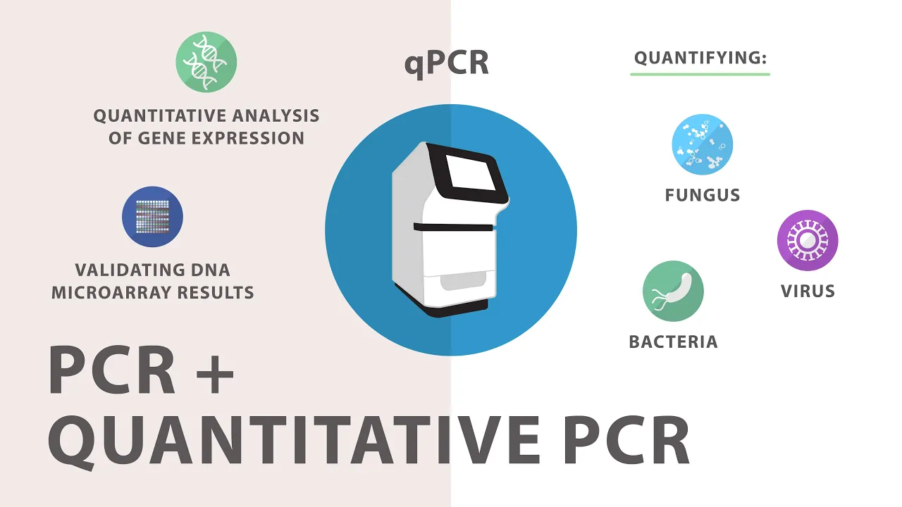
Quantitative real-time PCR (qPCR) is a molecular biology technique used to detect and quantify specific RNA molecules in real-time during amplification. The method relies on SYBR Green dye, which fluoresces only when bound to double-stranded DNA, allowing the machine to monitor DNA accumulation cycle-by-cycle. The cycle threshold (CT) value indicates the amplification point where fluorescence crosses a detection threshold, with lower CT values signifying higher initial template abundance. Data analysis uses the ΔΔCT method for relative quantification, comparing target gene expression against reference genes. Melt curve analysis verifies amplification specificity by monitoring fluorescence as temperature increases, ensuring only the desired product was amplified. Successful qPCR requires optimal reaction conditions, proper primer design, high-quality RNA/cDNA templates, and careful pipetting techniques.
Quantitative Real-Time PCR (qPCR): Principle, Method & Data Analysis
Added:this is a detailed video on quantitative realtime PCR stay tuned till the end and you would learn many things about quantitative PCR quantitative real-time PCR is used in research and Diagnostics to detect and quantify specific RNA molecules in the time of coid quantitative realtime PCR became really popular and every one of us has some idea about qpcrs or rtpcr so it has biomedical applications and it has applications in clinical diagnosis so let's talk about the qpcr applications in a nutshell so qpcr is used to quantitative analysis of the gene expression viral load pathogen detection genetic testing or even plasmid copy number detection now viral load detection and its example was very evident during the time of coid literally every everyone was undergoing a qpcr reaction right to detect specific viral viral DNA from their samples alongside viral load detection there could be gene expression analysis that is very evident for the scientist in biomedical Labs also qpcr can be combined with other techniques like chromatin imuno precipitation to analyze the transcriptor transcription Factor binding to a specific DNA segment so all these applications make qpcr a valuable technique for biologist that's why we should learn the technical details of quantitative PCR so question is how to set up a quantitative PCR and it's not really difficult to set up a quantitative PCR in the lab so let's learn the process these are the reagents required obviously we can we need to have DNA or cdna in this example it's cdna then appropriate primers forward and reverse primers dntps cyber green mixture and polymerase mix so basically cyber green is helping in the detection process and polymerase would help in the PCR reaction so this particular video talks about the Cyber green chemistry but there are other tman based assays which can also be used for quantitative PCR but the most used say is cyber green that's why we are talking about cyber green as well then the assembling all the reaction mixture is done in a tube or in a 96 well plate and it is loaded in the qpcr machine which reads these plate so what really happens inside the tube each of these machine has specific detectors for fluorescence so now let us look at one particular reaction and the Cyber green chemistry so this this is a DNA and cyber green is a Dye which is uh present in the solution and when it is in the solution and in in its Unbound format it doesn't flues but when it binds to the double stranded DNA it can flues and that is what is detected in quantitative realtime PCR so imagine this is the cycle number one in the PCR and you have to simplify things and understand okay we are only starting with one DNA but it doesn't happen in reality there are obviously more and more number of dnas to start with but in our linear example imagine we are starting with one DNA in the cycle number one so what happens in the cycle number two so there would be two copies of DNA right and obviously there would be a little bit more fluoresence compared to the first cycle think about cycle number three and cycle number four gradually the fluoresence levels are increasing because more and more DNA molecules are produced so obviously there are more die binding to the DNA molecules now let us look at this conceptuality in a graphical format so the machine displays this data as a relative fluoresence unit in the y- AIS and cycle number on the x-axis so what happens in the initial cycle the fluoresence level doesn't grow that much but after a point florescent level grows and Crosses a detection threshold and after that the reaction moves like a uh exponential curve so at a particular cycle number where the fluoresence uh reaches the threshold is known as the cycle threshold CT or CQ I'm sure that in coid you already heard about the CT or CQ values so let's see why this is important so CT value gives idea about relative abundance so this is the dete ction threshold imagine this particular red curve is corresponding to a gene a and blue curve corresponding to Gene B so from the CT value can you imagine which one has a higher abundance okay now if you understand it properly the abundance is high for the red Gene because its CT value is low that means it takes less amount of Cycles to reach the detection threshold if the is high there would be already more DNA to start with so it the threshold Crossing is quicker so basically the blue curve took more time to cross the threshold and now we are going to look at exactly the programs in the machine and how exactly that means so this is how a typical qpcr uh qpcr program look like in a qpcr machine so in this case you can see at 95° integrate what happens the DNA strand separates that is the denaturation step which is true for any PCR reaction then in the analing step the primers anal to the specific region dedicated for them to bind and the main thing happens in the step number four in this case so the extension while extending cyber green di also binding and that is the step where the machine detects the fluoresence after the reaction is over a melt curve analysis is performed and in a moment it would be clear why melt curve is important so imagine we have we have a qpcr graph like this and this we have done this for 30th cycle so of the 30th cycle the reaction kind of reached the plateau so we have this amount of uh DNA to start with then after that what happens gradually the temperature is increased in a 1° increment scale so this is called a melt curve melt curve uh kind of cycle so in this case what happens if we increase the temperature after a Time Point these products which are formed in PCR would melt down their DNA strands would separate and exactly at a particular temperature when the milk when the DNA strands separate we don't see fluoresence because the Cyber green then moves out and in Unbound State cyber green doesn't fluorescent so there would be a dramatic drop in the fluoresence that could be found in this curve so this is exactly known as the melting temperature now this is a graphical representation of the data that the machine spits out so here you can see there are three important type of curves so one one is the amplification curve that tells us whether amplification happened or not so you can see here there are two examples in this case in the left side you can see the cycle threshold is around 20 and on the right side you can see the cycle threshold is around 30 so the Cycles are basically on the x-axis so obviously you can understand which Gene is more abundant or less abundant then you can look at the Melt curve so you can see at a particular two of these genes doesn't have a similar melt curve the gene on the right hand side melts at 85° temperature look at the x-axis and in the left hand side you can see that melting temperature is somewhere between 78 or 76 something like that and obviously this melt uh curves can be visualized as a derivative the change in fluoresence over time so that gives us this kind of melt Peaks but question is what what is the importance of these kind of Peaks it turns out melt individual melt picks tells you that okay there is only one amplicon so that is really important to do at the end of qpcr it ensures that your amplification is specific and not halfhazard so let's talk about the qpcr data analysis it can be done by several method one of the most popular method is relative quantification by leac methods also known as Delta Delta City method so imagine these are the city values for Gene X that we want to detect from our sample and these are the housekeeping reference in this case it is 18s ribosomal RNA is the housekeeping so first we calculate the Delta C Delta CT simply means the CT values for every any Gene minus the CT value of 18s here note that on the uh uh left side there are samples from control and a mutant situation as well so for each of these samples the CT Delta CT values would be calculated after that the the average CT values can be uh determined basically control 1 and control 1 simply means there are two technical replicates that means control one two samples are not really biologically different they are exactly technically uh different so they are loaded two times just to have a uh kind of like a technical validation so that is why we average them eventually there is a calibrator that means uh the all the uh average of all the control samples so here the control 1 control 2 and control 3 Delta cities would be averaged as a calibrator then we will be having something called Delta Delta CT that means CT values minus the Delta CT values minus the calibrator values and you can see Delta Delta city is like that and finally the fold change would be calculated as 2 the^ minus Delta Delta City and this is uh properly known as leac method the paper link is provided in the description here you can see how the fold chain look like one can definitely plot it in a graph and from the graph you can see the control CT values or control fold change basically Falls near the range one so you can see the overall average is near one so with respect to control you can see there is a down regulation of that particular Gene X in the mutant scenario so this obviously gives us an idea about gene expression changes and which is super important for any um academician or a clinician in this case and you can also perform statistics like student te test and man Whitney test all of these to understand whether there is a significant difference or not now let us get back to the Melt curve amplification curve and melt curve so here you can see this is the amplification curve and this is the Melt curve or melt Peak analysis so here you can see there is this is the negative control which has a CT value far away from the uh normal any normal gen normal genes and whose melt Peaks are also shifted from the main cohort so this is something to check from your reaction so this is an example where the amplification curves looks okay but look at the Melt Peak so basically you can see there are many peaks in the Melt Peak that simply means this is not a proper reaction so this kind of multiple Peaks means there are non-specific amplification once you get these kind of data simply you have to optimize your primers so one this this melt Peck one and two simply means there are multiple products maybe one is corresponding to your non-space specific amplification one is your desired product so in this case one can use a technique called gradient PCR to optimize their primer in the gradient PCR using different uh gradient thermal block one can basically uh understand which particular temperature is optimal for a primer hybridization so instead of one particular uh primer analing step there are multiple uh temperatures which are assigned to the primary and Link step and it is done with a specific thermocouple present in the PCR machine later on one can run it on a gel to understand which is the desired temperature which give us best band for example in this case you can see 62.3 is a good particular temperature which give us a band and doesn't have other non-specific bands and it has a desired and significant yield you can see 49 or 50 has given several different bands due to non-specific amplification so that is why this is how one can optimize the prime and do their qpcr in a more efficient way so obviously what determines the success of a qpcr reaction these are optimal reaction conditions primer designing amplification efficiency quality of the RNA and cdna and pipeting efficiency all these factors matter for a successful qpcr experiment so I hope this was very useful if you like this video give it a quick thumbs up don't forget to like share and subscribe please share this video with your friends if you think it is useful share with your friends support our Channel using super thanks and see you in next video
Up Next

Gene Therapy Design Using AAV Viral Vectors | BHU Lecture
@APNAAMERICA
24.6K views•2025-11-10

AAV Production in HEK293 Cells: A Lab Protocol | NIIMBL
@innovatebio
2.2K views•2021-12-04

Affinity Chromatography Explained: His & GST Tag Purification
@animatedbiologywitharpan
45.2K views•2016-04-13

CRISPR and Genetic Engineering: How Gene Editing Works and Why It Matters
@kurzgesagt
30.5M views•2016-08-10
Related Study Plans & Knowledge Roadmaps
Structured learning paths in Biotechnology