




















Pre-whitening frequency analysis is an iterative technique used to measure the pulsation periods of variable stars by successively identifying and removing the strongest signal from a light curve, then repeating the process on the residuals until no more significant signals remain; this method uses periodograms to detect significant frequency peaks and applies significance testing (typically using a 5-sigma threshold) to distinguish real pulsation signals from noise, enabling astronomers to extract multiple pulsation frequencies that reveal information about stellar interior structure.
Python Variable Star Frequency Analysis with Pyriod
Added:Basic Stellar Astrophysics: Understanding variable stars, particularly pulsating variables, and how their physical properties relate to periodic changes in brightness (light curves).
Foundational Time-Series Analysis: Understanding Fourier analysis, periodograms (specifically the Lomb-Scargle periodogram), and how time-domain data is transformed into the frequency domain.
Core Python Programming: Proficiency with scientific Python libraries such as NumPy, Pandas, and Matplotlib, which are essential for handling and plotting astronomical data.
Signal Processing Basics: Understanding the concept of noise in observational data and the general objective of 'prewhitening' (removing dominant signals to reveal weaker ones).
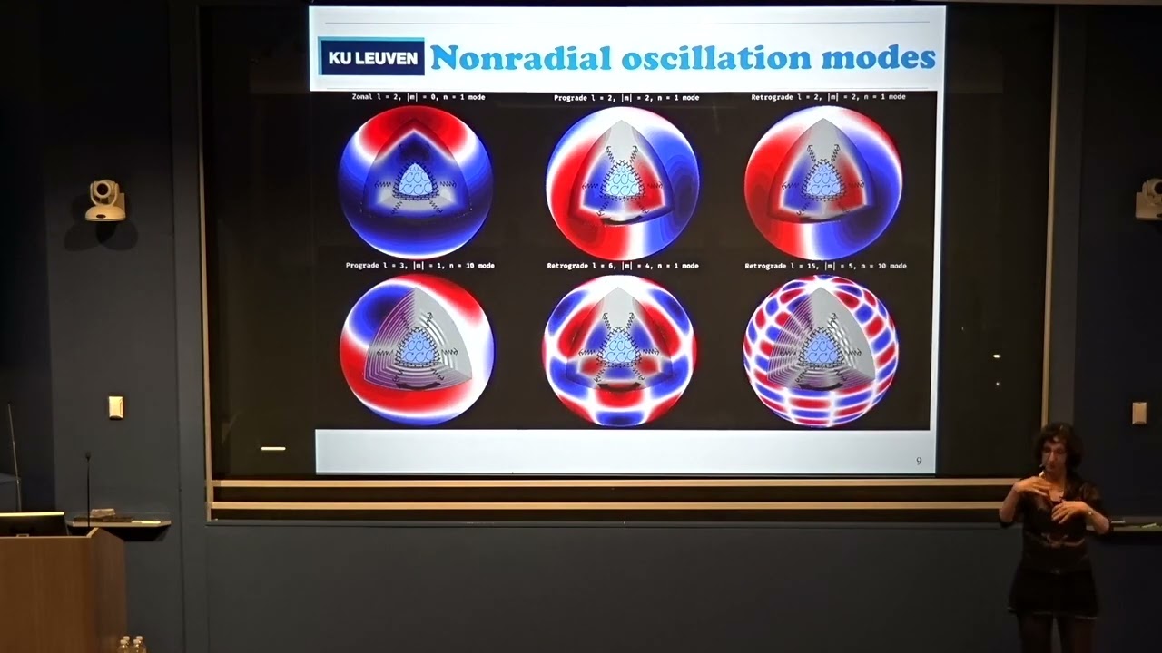
Introduction to Asteroseismology: Utilizing identified pulsation frequencies to probe the internal structures, density profiles, and rotation rates of stars.
Space Telescope Data Processing: Applying these frequency analysis techniques to high-precision light curves from missions like Kepler, K2, and TESS, including handling instrumental systematics.
Advanced Modeling of Multi-Periodic Stars: Studying non-linear mode coupling, amplitude modulation, and the physical mechanisms behind multi-periodic stellar variations.
Large-Scale Automated Pipelines: Scaling up period-finding techniques using machine learning or automated algorithms to analyze millions of light curves from upcoming surveys like the Vera C. Rubin Observatory (LSST).
2.7K views58likes1:10:46Original Release: 2022-10-12
registration is open for our 111th annual meeting and this year's annual meeting will be held on November 4th through 6th in Tucson Arizona we will be broadcasting the meeting online simultaneously in order to provide interactive experiences for both in person and online attendees registration for the annual meeting will remain open until October 25th and remote attendees may continue to register until October 31st but if you're planning on attending in person make sure that you get your registration in by the 25th all right now we would like to thank and acknowledge our sponsors voice Astro and chroma technology The Voice research initiative and Education Foundation provides online astronomy education Observatory resources and research experiences to students student teams and schools in order to learn how to perform observations conduct research and publish the results in scientific journals such as the Journal of the aavso please check out their webpage to learn more about their work founded in 1991 as a 100 employee-owned company chroma technology is a leading manufacturer and OEM supplier of Highly precise Optical filters using thin film coating technology their reputation is built on dedicated customer service including free Technical and application support they remain committed to serving both the scientific and Technical communities in their pursuit of the scientific endeavor chroma's product portfolio provides solutions for Industries ranging from the life sciences and agriculture to manufacturing inspection security and Aerospace the broad array of applications served includes fluorescence microscopy flow cytometry biomedical instrumentation surgical devices Machine Vision multi-spectral Imaging and of course our favorite astronomy hey now let's go back to this title slide here our instructor for today is an assistant professor at Queen's College of the City University of New York an expert on white dwarfs and time series photometry he spent hundreds of nights shooting time series out at both McDonald Observatory and Apache Point Observatory he also has extensive experience analyzing data from recent photometric surveys including Tess Kepler and this Vicki transient facility a couple years ago he created the python package pyrid which is used for pre-widening frequency analysis of Time series astronomical data if you're interested in analyzing data mined light curves or doing Astro seismology on your own computer a pyrated may just be the tool for you fortunately we have only the best of instructors here with us today to teach us all about the ins and outs of pyrid and how you can use pyrid to do science personally I can't wait to learn more about it so without further Ado please allow me to introduce our instructor for the day Dr Keaton bill welcome Dr Bill thank you hello variable star observers I'm excited to be talking with you I'm going to share some tools and techniques today for measuring the variability periods that are present in the light curves of variable Stars we're going to do this in a python environment making use of some interactive tools that I've developed this pyria package that was just mentioned so most of this will focus on how to use pyria to do what's this so-called pre-whitening frequency analysis process which I will explain but first i'm going to introduce you to the Jupiter notebook environment for running python code uh so let me share my screen here [Music] what you're seeing is a internet browser if you attended the last python webinar you would have seen how to use Python from the command prompt as well as how to write and run code that's written in a file but for this tutorial I'm going to use this this other programming environment called a jupyter notebook that's spelled Jupiter with a py in the middle for python and I brought this up in my browser on my Mac computer by typing into a terminal the words Jupiter and then notebook and that brought this window right up in my browser if you're on a Windows machine and you've installed python with Anaconda distribution then I believe there should be a Jupiter notebook icon in your start menu somewhere that you can just open it right up from there Jupiter notebooks are a great programming environment for learning to code especially because you can write your code and run it in in blocks at a time these code blocks are called cells and it works all right inside your internet browser so this is this is what I see when I open up a jupyter notebook in this folder that I created for doing this tutorial it shows all the files that are located in my folder I've got a fits file a CSV file a PDF and then this dot i p y and B file this is an interactive python notebook if I click on this it's pretty much empty I've just created one for this tutorial and I wrote some information up here and just plain text to describe what the goals are for today there's a little bit of information about this python package pyrid which you can read more about on this link that's used to analyze light curves so uh to install pyrid on your own machine if you want to do this you've got to run this pip install pyrid command in your command prompt or your terminal that will install the software so that you can import it and use it in Python and then because this code it involves some interactive widgets and buttons for uh manipulating and inspecting your data interactively within your browser you have to enable these notebook extensions that allow you to do these things so you would also run these three commands after you've installed pyrid and before you open up your Jupiter notebook in order to get it fully installed that information is all on the pyrid website so this is just some information I'm going to press this plus sign to insert a the first code cell here's where I'm going to write python code and the first line that I'm going to write is another sort of specific to pyrid line to help that work and to display all the widgets and buttons that we want to use it's a so-called magic python command that starts with a percent sign the right mat plot lib which is the plotting library that I use space widget and that will allow me to use the widgets that come packaged with pirates and then I will also import the other packages that I'm going to use the first one and I'll show you some of the capabilities of this package is called light curve with a k that K stands for Kepler which was a photometric mission that you may be familiar with this package was originally developed to work with and manipulate and analyze light curves from the Kepler Mission but it's now used for all sorts of light curve data that you could get especially data from tests which I'll show you some of in this tutorial uh so we'll import light curve as LK just to shorten the name of it a little bit and then for pyrid I'm going to import from Pirates I'm going to import hybrid because that's just a little bit nested in there uh we can run a cell of code in a Jupiter notebook by holding down shift and hitting return and this the last risk means the code is running and then once you see a number there the code has successfully run so in this environment it's just like if you had typed this into the command prompt we've now imported these packages for use um these are the only these are pretty much the only two packages I'm going to use for this tutorial there's really not going to be a lot of programming that I'm going to do we're going to use Python Programming to get the data into the pirate interactive analysis environment and then we'll carry out the analysis by working with the buttons that that provides light curve lets us work with all sorts of light curve data and it has a lot of great functionalities that built in the one I'm going to show you right now is that it can it can actually be used to search for and download archival light curve data from the Kepler or test missions and then I'll also show you something great about uh about Jupiter notebooks and why these are so helpful for learning how to program is you can use tab complete to see what's available so for example I've imported this package like curve as LK and now if I want to know like what functions like curve makes available to me I can type the name of the package and a DOT and then if I hit tab it brings up a whole list of functions that are available to me in the light curve package so this can do all sorts of things what I'm interested in doing is searching for a light curve so I'll click on that the Searchlight curve function that's the first you know just a super powerful thing about Jupiter notebooks as we can see what functions are available to us by hitting Tab and then the next most useful thing for learning python is that once you put these parentheses here as long as your little you know the little blinking line is here inside the parentheses if we hold down shift and hit tab I like to hit it twice then it will show us what the what the calling sequence is for this function this LK dot Searchlight curve function takes a required argument which is the target it's required because there's no equal sign there and then it takes all these optional arguments these have default values and if you scroll down here you can read the documentation for the function it tells you what kind of parameters are allowed what what this function is going to return a search result and give some examples so all this documentation is at your fingertips with jupyter notebooks I'm going to search for the light curve of a legendary pulsating star Essex phoenicius okay this is like a high amplitude Delta scooty sort of pulsator and I run the cell by holding down shift and hitting return and this shows me a search result with 11 data products okay these data products are all from tests data they're created by different authors the SPOC products these are sort of the the main test pipeline products but there are also some other pipelines for extracting light curves from the test data and so you can see that that those are available here as well and this star was observed by Tess in sector two and in sector 29 sector 29 this was during the uh kind of the extended mission for tests and there's a couple different modes of data during sector two there was short Cadence data where the images were saved out every 120 seconds and then there are light curves extracted from the full frame images that were read out every 30 minutes in sector 29 there was also this Ultra short Cadence which is a 20 second Cadence light curve and then the full frame images started to be read out every 10 minutes so even faster at the at the slowest rate there we'll just pick one of these to download we'll pick the first one the 122nd Cadence data from sector two and so I I select this this is a an indexed list of results I'm going to use square brackets put a zero here to select this one uh this this one product and you can rerun uh you can rerun code in the same cells to to manipulate what is available what what's stored in different variables in Python here once I've selected which data product I want I'm going to press a period you can hit tab to see what functions are available to me now and there's a download function so I'm going to use that one to download this light curve and here is the light curve data there's a bunch of different Columns of different information I don't know what half of these are but the ones I'm really interested in for my light curve analysis are going to be time right these are time and some sort of fractions of days relative to some reference state flux in physical units of electrons per second and an uncertainty on the flux the flux error you see the flux here in physical units is sort of this is scientific notation so this e e plus whatever says how many zeros have to go on to the end or how many spaces to move the decimal point these are sort of in the 200 000 counts level for a light curve I'm not interested in this analysis and exactly how bright the star is in each measurement I want to know the relative brightness how is the brightness varying relative to the average brightness of the star and so I'm going to do one more thing the way light curve is written you can really write these functions with like like a sentence like this is a star that I want to download and then I want to normalize so that the average value is one and the fluxes are relative to that so here e to the negative one this is like 0.96 this is 96 of the average brightness up here uh towards the end of the table this is like uh 22 as bright as average so we're seeing this uh this light curve data and manipulating it in a table um what I what I really want to do here is now I want to store this in a variable and I'll call LC so that table with all that data is stored in this variable LC and then I can pass that to the like sorry to the pyrid package and create a pirate object so I'll call this object lowercase pirate see that equals Capital Pi red that's the function I imported from the pyrid package and I'll pass to that because in the uh a net signature here to initialize the pyrated objects you have to pass a light curve object uh from the light curve package that's what we just downloaded so I'll pass that here and we've created this light curve object we can start analyzing this data set to do that lowercase pyrid dot again Capital irid open close parenthesis and this displays this interactive cell for inspecting and fitting and manipulating this data set so we see this beautiful time series light curve here this is a richly pulsating star observed by tests we can zoom in and see the beautiful pulsational variations here it's just an incredible data set um and uh this is what we are going to fit a model to what we want to do is measure all of the frequencies that are present in this data set because of the frequencies of variability here are pulsational frequencies of standing waves in this star and the standing waves in this star these sensitively probe the interior structure of a pulsating star and by measuring many frequencies of pulsations from a star like this we can potentially constrain the structure of the interior and you know probe the physics of the interior of this type of star so that's the that's the science goal for this type of analysis and for acquiring this type of data but how do we do that well the pre-whitening frequency analysis technique utilizes sort of two views of the data there's this time series view measuring the relative variation over time but there's also this periodogram View and in this tab you see what the frequency content of the data is so there are all these different lines that kind of stick up from the bottom axis these indicate that there are significant frequencies of variability at each of these values what the periodogram does is it tests for a full range of frequencies that these data may be sensitive to it measures how large of a sinusoidal variation at that frequency would best fit to this data set so for example you see that overall there's sort of uh you know a periodicity here there's something that's generally repeating sometimes it gets a little higher sometimes it's a little lower but there's a main a signal running through all of this that's going to correspond to this highest peak this is the dominant sync signal in this data set this this black dot here allows you to select different peaks in the periodogram and it started at the highest signal this is in units of micro Hertz for the frequencies those are how many um so those are a million times smaller than a um than a Hertz so this time scale of around 200 micro Hertz that's like a little bit more than an hour you can also set when you create this pyria object there's an option to change the frequency unit if you prefer per day or amplitude unit if you like percents or something like that but this in parts per thousand 140 parts per thousand there's a variation at 210 micro Hertz of about 14 variability and indeed we see that these highest peaks reach up to kind of 35 percent uh brighter than than average uh this is the dominant signal here so what I'm going to do for my analysis is we're actually gonna carry out this um this pre-whitening process which I've created this flow chart for and we're going to ask ourselves these questions right is there a significant signal in the data and we're going to ask that just about one signal is there a significant signal in the data here I see that this peak stands out way above everything else that is a significant signal in the data so the answer is yes this little flowchart tells me to Stage this signal frequency for fitting so I'll show you what that means that means I'm going to add this signal to my frequency solution I pressed that button and that put it into this interactive table that's located under the signals tab in the signals tab we've now just have these These are starting values that came from the periodogram just the location of the peak here the frequency is about this the amplitude is going to be around this value but there's no measurement for the phase this is the signal of a sinusoid a sinusoid has an amplitude a frequency that it repeats at and then a phase that that just shifts it uh in line with the data set these are just initial fit values but we can actually fit this to the time series data by hitting refine fit and this finds the best fit phase value it also Returns uncertainties on the measured frequency and on the amplitude because these are such Exquisite space-based data we have really precise measurements of the frequencies this is 210 micro Hertz but it's it's measured to a Precision of uh I don't know what this is a terahertz I think so many orders of magnitude uh signal to noise here the amplitude is also measured very precisely and if we go back to the time series tab and zoom in a little bit because this this data set so long we see the model that's currently fit to the data in red and so we see that it is it is repeating at the right time scale of the main variation that's present in this data and it's also reaching its Peaks at around the same time that the data set here reaches its Peaks um that's that's very good so I'm sorry I've I've skipped ahead in the flow chart I that was the step to refine the fit to the time series and then we have to ask ourselves another question similar to the first are there more signals in the residuals well let's talk about what the residuals are first the residuals are what variations uh remain after fitting this model that is it does is there anything left does this model leave anything to be desired uh for for obtaining a perfect fit to this data set I would say yes it does this this model does not produce these very high peaks for example we can see the difference between the model and the measurements by plotting the residuals we zoom in here we see this is a little different this we've removed the main signal but this all this variation is still present in the data and we we should take efforts to include all of that in our solution as well if we look at the periodogram again uh looks similar to before but the signal that we included in our frequency solution is now colored green and all the other signals are blue that's because we've included that bit in the model and that's the periodogram of the model and in blue we see the periodogram of the residuals that's what remains to be fed um so these we can we can see what's in the model our model right now is just a single signal and in the residuals there are a number of Peaks that correspond to signals that we need to include uh in the residuals to account for all of the variations in this data set this little black dot goes to the uh the highest peak in the periodogram of the residuals and we can repeat this process so this is this is ready for us to add to the solution we can click that button right that's in our table here now and we can refine the fit to that signal we see that that Peak has turned green it's been moved to our frequency solution and the time series plot uh it's a little peakier now it's getting a little closer to reproducing those uh high flux excursions um but it's still not perfect uh and sure enough there are still plenty of signals to be included in our model here so we continue the process add to the solution refine the fit add to the solution refine the fit you see these Peaks are turning green as they enter our frequency solution then we can continue this uh on and on and on but at some point we'll need to stop and we need a stopping condition so let's see here so in order to do that we need to compute a significance threshold there is this question in the flow chart or this um hear about significance and the fact that we are looking for signals in the data signals as something distinct from noise all of our measurements will have Some Noise associated with them we saw the flux error column of the light curve earlier there's uncertainty on our measurements and if we Zoom way in down here on the plot the periodogram of the residuals you see the remaining Peaks are are standing out above sort of a a baseline level of just Little Peaks everywhere right these are noise Peaks these really small ones um these represent uh what's needed you know there's a lot of different sinusoidal frequencies that you would have to introduce to your model to not just fit the pulsation signals but to perfectly reproduce every single data point which includes the noisiness of the measurement and we don't want to include that in our frequency fit because the frequencies that we measure for the pulsating Stars we want to interpret those as the frequencies of Stellar pulsations things that reveal the interior structures of the star and if we include a noise Peak our noise frequency in our analysis it could we could really misinterpret what's going on uh with with this object we're interested in so we need some way to tell the difference between a real Signal Peak in the light curve and a noise Peak and the typical way of doing that involves something called significance testing uh or or sorry it involves something called hypothesis testing uh we are we are testing for significance um but to decide whether peaks in this periodogram are significant we're going to adopt the hypothesis that all of the Peaks that remain in the periodogram of the residuals that all of the the whole periodogram just represents noise let's just adopt that hypothesis and then test that hypothesis and see if we can reject it if we can reject the hypothesis that there's only noise remaining in the residuals of our model fit then we can then we know that there must be some remaining signals in order to describe the data so the hypothesis that the that the periodogram here only only has noise in it uh that implies that most of the variations here I'm going to hide the model right now that all of these Peaks uh are at a similar size to each other and that uh it's a property of noise in the periodogram that noise Peaks pretty much never stick out more than five above more than five times the average noise level in the periodogram so and that's just kind of a rule of thumb number that I use for space-based data some people use different scaling factors for their noise significant thresholds but what we can do here is we can use the significance threshold functionality to calculate the average noise in a sliding window across the periodogram and then multiply it by this factor that five times the average noise I'm going to say that's as high as a noise Peak should ever get so under the hypothesis that this periodogram only has noise peaks in it I should be able to calculate this significance threshold and see that nothing exceeds the dashed line well this exceeds the dashed Line This exceeds the dashed line there's all sorts of stuff that exceeds the dashed line I have to reject my hypothesis that this is just noise in the periodogram and since I reject that hypothesis I say well then there must be signal in fact all of these things that stick out above five times the average noise background must be signal so we can add these to our frequency solution sure enough I'm I'm disappearing these from the plot they're going into the model add this one to the solution etc etc now at some point the highest peak ends up being very close to zero in a lot of cases this is zero frequency this is not actually a pulsation frequency of the star but it's it's trying to capture a little bit of this very slow variations uh that are systematics in the test data most likely so I'm not going to use the frequency here at one micro Hertz there was suggested to me instead I'm going to click over here and select a different different frequency to add to my growing rapidly growing list of pulsation signals so I can add this one I can add this one there's really a lot of signals in this richly pulsating star we're not going to get to the bottom of this during this talk this could I could I could go on like this for hours probably finding new signals to include in the model but what I definitely want to show you is that our model fit to the time series data is really improving at this point we are really reproducing these variations and we're building up a a large table of pulsation frequencies they're corresponding amplitudes their phases we've got uncertainties for all these measurements this is the kind of data set that we want to produce for uh these are the type of measurements we want to produce for such a beautiful data set like this this test light curve of SX finishes um as we add these signals to our frequency solution we can also go ahead and um recompute our significance threshold because we've removed things from the residuals periodogram and that will lower the significance threshold making even more Peaks statistically significant and worthy of being added to our frequency solution there are probably over a hundred signals in this data set that are significant and that we could analyze to learn more about this star so I'm not going to add all of them in fact I'm going to uh to stop adding signals and just show you this result you can imagine the the continuing to to include uh additional frequencies will help to fit some of these remaining residuals which you can also look at in the time series tab you see that this isn't just noise there's correlations among these points you can kind of see by eye although it's getting harder as we go to these really small amplitude signals see that there's some additional pulsational variability here but we're approaching a nice measurement of all of the periods for this star so I've just got a few more minutes and I want to show you one more thing because this is a aavso seminar um I thought I should look at some aavso data and especially show you you know how you could get your data or any time series data set into pyrid for analysis not just the things that are downloadable through light curve so I'll do this really quick I already downloaded and sort of manipulated uh the aavso light curve for SX phenicious the same Target that we just looked at the test data for I'm going to import just one more package here that I'll use to read in the aavso data I think in your last Python tutorial you saw how to read in a CSV file a light curve from a CSV file I'm going to do the same thing here store as a data frame just using this read CSV functionality the AAA yeah so light curve uh this is a table similar to the one you saw before there's dates there's well magnitudes in this case not flux there's uncertainties there's a bunch of other columns right Observer affiliation somewhere in here's the name of the Observer who should probably get credit um and I'm going to pick out the columns that I'm interested in and I'm going to turn them into a light curve object so light curve sorry first I'm going to uh pick out the columns I want this is a date column I'm going to call this time time and there's also a there's a magnitude column I'm going to convert this to a flux I'm not going to worry about the scaling Factor too much because I'm going to normalize it so I'm going to take this 10 to the which in Python is 2 2 multiplication signs 10 to the negative 0.4 magnitudes I think I hope and call that blocks and I can pass this to an LK dot light curve object with those capital letters in there this can be passed just a whole data array or it can be passed the time flux and flux error columns I'm not going to worry about flux error right now because I'm just trying to demo this say time equals time Lux equals blocks you could add flux error if you wanted but this creates a light curve object they always have these three columns time flux and flux error by the way light curve is a very powerful tool for working with this type of data so if you want to learn more about that you can go to light curve with the K dot org and they have some great tutorials and demos about the capabilities of this this package I really recommend it it's a great package it's really made doing science with the light curve data a whole lot easier and it's what pyrid uses behind the scenes very much to do its calculations I'm gonna call this lc2 because we already have something called LC I'm going to pass that to something I call pyrid2 because we already have a object called pyrid lowercase pirate pass lc2 that and look at the interactive hyriad tools um now this isn't all the avso data that's available for this star I just selected uh two nights of data where there was quite a bit of measurements uh for this star and I selected just the v-band filter uh you know what there's one more thing I want to do here I'm going to normalize this light curve and then I'm going to pass it to pyrene2 and redo this so now it's kind of relative variations compared to the the average uh if I zoom in you can see what the aavso data captured on the first night sort of is about two hours of data probably uh captured a couple of cycles of the main pulsation signal and then about 30 days later there's about a cycle and a half that got captured here so uh well will the data quality during the observations look quite similar to the test data quality uh there and and the duration of the light curve is about the same there's obviously many days without observations here which is going to make this data set more difficult to analyze as you're about to see because if I look at the periodogram here these peaks look way wider there are there are Peaks that stand up above the the background of of signals but each of these features are sort of filled in a little bit more compared to up here where when we looked at the periodogram of the uh when we looked at the original periodogram the highest peaks were like razor thin uh because they're so precisely measured measured with so much data these Peaks are much wider because each each observing run was only a couple hours and that kind of sets the width of these signals that's sort of how precisely we could measure these frequencies it's pretty limited by how short each individual visit to the star is if we zoom in here see there's a little bit more going on and if we zoom in even further we see that there are actually these sort of like a lot of Peaks all over the place like a big zigzag pattern and you could pick any of these highest parts of the periodogram to add into your frequency solution and the problem is knowing which of these to include if we pick the highest one here and we add this to our frequency solution we get a good we get a fit a very precise error in this case this doesn't really represent the uncertainty because it only measures the the sort of the width of this one particular Peak it's how precise we could measure this signal if we knew that this was the correct Peak um but what but you see that um what's gone into the model even though we only selected one Peak uh to include in the model in the periodogram of the model that that has taken away the power from all of these Peaks that exist here and that's because uh each of these uh each of these Peaks basically represents the same signal they each they fit very nicely any of those frequencies would fit the main variation on this first night of data quite well they would each fit the main variation out here quite well but all those Peaks appear because of this huge gap that we have we don't know because we weren't looking how many exactly how many cycles of pulsation we missed during those 30 days when observations were not being taken for this star so uh that's what each of these Peaks corresponds to you know there are many hundreds of cycles that we missed and there's a peak here that corresponds to missing say 400 Cycles when we weren't looking and then there's a peak that corresponds to say missing uh 399 cycles and 398 Cycles at 401 Cycles 402 cycles and that's uh something that our data are not sensitive enough to tell the difference between so that highest amplitude signal that we found here um the one that was just automatically selected was 217.9 so let's say 218 micro Hertz from the test data where we didn't have the problem of all these Peaks these Peaks are called Alias Peaks over here the ones are they're very small and right next to the the main Peak here we were able to measure that the strongest signal was at 210.57 micro Hertz so that must be the same signal that we're looking at but we picked out this the wrong Alias peak in the periodogram I'm going to delete this from our solution to go back to the beginning where you can see where all of these different Peaks are I'm going to look because one of these is going to be I think this one here at 210.57 micro Hertz that's matching the signal that we measured so precisely from the test data so when you're looking at ground-based data this is the Big Challenge if you want data that spans a large Baseline so that you can measure the periods that are present very uh very precisely but you also don't want very large gaps in the data because that limits how accurately you can measure the pulsation frequencies or whatever frequencies are present in your data and that affects how good your results will be so without any other data it would be impossible for us to choose any one of these frequencies as being the most significant but because we can reference the test data which was able to resolve the correct signal we can confidently add this frequency to the data set and then we could go and look for additional uh significant signals in the residuals in this case I think it would be difficult again to pick out which of the many Peaks that are part of this uh set of signals is is potentially the real one um so I'll show you one last thing that that pirate is capable of maybe some of you with Keen eyes notice this um the first frequency I added was 210.57 micro Hertz the second frequency from the test data was 421.14 micro Hertz that's two times this value um so I I was sort of misled you this is not actually an independent pulsation frequency it is a signal of the pulsations but because it's exactly twice this frequency uh we call it a combination frequency or a harmonic signal it doesn't represent an independent a standing wave pulsation frequency in the star um but knowing that this knowing something like the second strongest peak in this star has a frequency of exactly twice the strongest Peak allow it gives us a way to pick out the correct signal in the aavso data where there are normally many candidates we can pick out the one that's twice the signal that's already included here or with pyrid we can actually just Define the frequency to be a mathematical mathematically related to the frequencies that are already here we could call this two times F zero and we can add that to our solution so this F 0 and 2 times F zero this frequency is always going to be exactly twice this if we type refine fit here we get a improve fit to the time series which now fits a little better than it was earlier um and Beyond this I think the aavso data it would be difficult to to measure any frequencies reliably beyond that but we've captured the two main signals that are present here from just uh you know few hours of data separate you know over the span of of a month so that's everything I wanted to show you for this talk but I welcome your questions and uh thank you thank you for joining today thank you so much Dr Bell that was an X excellent presentation very clear okay we have had several questions come in here already so um let's start with this question from Charles cinnamon who had asked about um aliasing specifically with regard to test data is that something that someone needs to be careful to uh care about and understand when working with space based data yeah it is so I mentioned a little bit about aliasing at the ends it's not exactly um I think what was being asked but this issue where there are where a sing a single this is like a tongue twister where a single signal uh it can cause multiple Peaks right there's only one frequency in the data but it's causing there to be like I don't know a thousand Peaks here or something right and selecting the right one is uh is one of the main challenges of doing this type of analysis now um that's not as much of an issue this particular type of aliasing that comes from the large gaps in the data that's not so much an issue for tests but there's another type of issue um let's take a look here there's another type of issue potentially in the test periodogram I'm going to recalculate this periodogram but out to a higher frequency than I did originally I let the program kind of pick a good frequency to use [Music] um let me see I remember how I even wrote this I just yeah um so restarting this analysis if we look at the periodogram now I've calculated it out to a higher frequency and you see more Peaks out here at the really high frequency um this is called Nyquist aliasing and this is where you um you need to be concerned a little bit that at least the data rate that you're getting that the the Cadence of the data or the time spacing between the data is sufficient sufficiently fast to resolve the the time scales the variation that you're interested in so if a star varies I do a lot of work with pulsating white dwarf stars so say pulsating white dwarf stars very um on time scales you know between a couple and maybe 10 minutes something like that so let's say a star we know a stark can vary as fast as every two minutes we know the type of variable we're looking at the time scales that might be relevant if the Stark can vary as fast as every two minutes we need to make sure that we're measuring uh these Peaks that we're sampling that time scale of variation which means to sample that well we need to have at least two data points per period uh so that we see the data both go up and then back down during that that brightness variation um if the data aren't aren't sampled finely enough uh then we might not be sensitive to that what you're seeing here is what's called Nyquist aliasing where every signal like this signal is mirrored over here this is another Peak corresponding to the same signal this is another Peak corresponding to the same signal now because of this uh duplication of Peaks by default pyria only shows you the periodogram up to the highest frequency that it would be sensitive to that the data are sensitive to but if the highest frequency the data are sensitive to is not as fast as the frequencies that are present in the data then what you see in the period the peak that shows up in the periodogram is a so-called Alias that the real peak is up here in the high frequency part of the periodogram that isn't uh usually where you're searching for signals but you probably identify the low frequency Alias and fit that instead I think pyria doesn't do a great job of showing you what these high frequency fits are you saw with the fit at low frequency looked like I'm going to try to um fit the signal and just see what it looks like in the time series tab it's it's a little under-sampled here you know when I saw when I fitted it originally you saw it it kind of follow the main variations here um right now what it's trying to do and it's not sampled finely enough but it it's basically between every data set it's going through a big dip it's because you're not constraining those frequencies of variability so it's it's like it fits through the point and then it it Wiggles and then it fits to the next point and then it does a wiggle and then it fits through the next Point uh and if you pick the one that was up here it'll do a couple Wiggles but you saw when I added this signal to the to the frequency solution it's not only this line that turned green and disappeared this one went with it that one went with it if you calculated this to way higher frequency you would see me you would see additional Peaks that are aliases as well that's a great question aliasing is a concern you want to make sure that the data sampling rate is fast enough for the variations you might be interested in and that's why when I first looked at this set of light curves that we could be interested in I picked the 122nd Cadence data instead of the half hour Cadence data because I knew we would need this fast this faster data set would be more sensitive and more accurately represent the variations that are present in this scar great answer thank you this one comes from someone who says they're a physics undergraduate student currently doing a project all about searching for periods of binary stars and for their project they've been using loam scargle to do the python code and they would like to know why you would choose light curve over loam scargle um this is a lot this is a long scarvel periodogram so um the type of periodogram that's being calculated here uh yeah I didn't use those words uh there's the time series uh I regret doing what I did here but uh yeah this is the um this is the long scargle periodogram um of this time series data so I think maybe that answers the question and it's computed right out of uh light curve so there's like you know lc2 is a light curve object um the light curve with the K package is great if I hit Tab and see what functionalities are here uh for manipulating this light curve object one of them is um is two underscore periodogram and if I put the parentheses here and look at the documentation the the default method for computing the periodogram is lomscargill and this is the function that I call behind the scenes in the in the pyrid package so yeah okay makes sense thank you okay and um next question here this one comes from Richard Wagner who says excellent I can't wait to move on to this from period 04.
um when analyzing a star would it be correct to manually input a bunch of the harmonics of the main frequency and then proceed to find possible other pulsation modes that way yeah I like that idea um I like the idea Richard and and I this is uh my homage to period 04 I use period 04 in my research extensively and then I kind of moved to python as that became more popular for doing research and I felt that a period of four like program was really something that was missing and you know we python is so great because people make available the tools that they're that they're working on so we've got things like astropi light curve package and uh and now uh pyriad is is my little pre-whitening contribution to that so I I just like the tabs here you may have noticed this is kind of similar to the to the period 04 setup so I was trying to replicate that um I think it is a great idea to try to uh input a bunch of harmonics um that that's I usually do it the other way I usually fit all the signals that are present and then once I have a big table of signals I sit down and I look and I try to identify okay this looks like a harmonic this looks like a because it's not just harmonics like multiples of a frequency sometimes there are combination frequencies that are sums or differences of multiple frequencies so you also have to look for that um but uh yeah you could start as you go that's a great uh way to do it if you because what I usually do is once I have the fits in here I do actually want to fit them in the model where I'm enforcing that the that the harmonic is frequency is always exactly twice or three times or whatever the the base the fundamental pulsation frequency or that the sum of frequencies that is always is exactly the sum of the involved frequencies and so I would prefer to write these in here like I've added this frequency I would prefer to put the next one as 2 times F0 add that because we know that's the next highest peak that's caused this signal to go away we could look for you know we could even sometimes I do do it this way 3 times F0 let's see if I add it here it'll put a little box there and sure enough there's one right there um so we wouldn't that the best way to include this peak in our solution is as a three times F0 we could refine that fit and as we fit other independent frequencies we could also try things like let's let's add this next Peak here to the solution we could explore to see okay I wonder if uh F 0 plus F1 is present we can add that to the solution and before we fit it we can just look to see oh yeah I that's um that's this one here that's still blue but has a little uh diamond on it and in fact all these uh all these orange diamonds indicate the uh combination and harmonic frequencies that are defined arithmetically and the uh the green diamonds are the independent frequencies so since this peak stands out above the noise I would yeah prefer to include that as F0 plus F1 and fit it that way great question great answer thank you okay um let's see so uh Joyce guzik had a question which I think is is pretty related to what you just talked about um does pyrid have a way to find all of the combination frequencies it does not currently have a way to find all the combination frequencies submit uh bit uh challenging a lot of potential combinations um but it's something I have in mind to try to implement it would be a really nice feature um so yeah possibly in the future we could try to do something like that okay thank you and uh next question here um are there any tutorials for installing pyrid from GitHub since a lot of us here are not actually familiar with installing packages in that way yeah um well you don't need to install it straight off GitHub you could as you're right I'll click on the link here and show you what this brings up so GitHub is a way is a place to store and store software and to distribute software and you could download it directly and install it with this setup.python function but I recommend this is also available on a on a package package manager pip so you can just type in your command prompt or your whatever you call it on Windows the Powershell or The Terminal depending on what type of computer you're on you can type this pip install pyrid line into your command prompt that should install pyrid for you but be sure to run these functions as well to enable the uh the widgets and also you need to type this line as the very first line in your notebook this matplotlib widget with the percent sign otherwise all of this stuff will not display and so you'll run your pyrid cell and this stuff just won't be here and so it's very important to install this correctly so those are the installation instructions you can read them here and it should just be these few lines pip install tie Ridge and then this and to your more specific question this is how you would install it if you wanted to download the version on GitHub you could download a zip file of the package and and install it this way but I really don't recommend it okay thank you okay um of time for I think about so um we had a question come in here from uh Ed Mullen who asked so all of these uh patterns that you've been finding and fitting what are they physically related to what's actually going on in the star to create this yeah these are um well I'll be honest this isn't the type of pulsating variable that I usually work on it was just a very nice rich data set to show you but uh so uh we'll allow my depth here but this is a pulsating variable star so each of these variations but more specifically the variations that are not um not these combination frequencies so in this set of of signals here um this peak is a pulsation frequency it is a resonant frequency of this star it's like if the star or a bell and you were to ring it this is a a tone that you would hear right and just like with bells if you were to ring like uh you know a a small jingle bell and you were to ring a big old gong those sounds would be really different those those frequencies are very sensitive tracers of the physical configuration of the object and so when you hear a bell ringing right away you probably have an idea of like oh someone's ringing a small little bell or someone just rang a big old gong you know you can right you're doing uh this frequency analysis in your head right and you're inferring something about the physical object that's vibrating we try to do the same thing with these pulsating Stars this is but these objects can can vibrate in many simultaneous frequencies that really help us to to to study and constrain the physical properties of these Stars so here this peak we're measuring one of the one of the resonant frequencies of this object here we measure another resonant frequency of an OB of the object these Peaks these these yellow diamonds that are the combination frequencies those have something to do with the interactions between these modes or the ways that uh that these modes both um affect the star as they as they read through it and so these are not independent pulsation frequencies but these two are independent resonant pulsation frequencies that's why it's important to identify the harmonics and combinations and distinguish them from the um I'll call them the the parent mode frequencies uh because the parent mode frequencies are the real uh you know bits of information that we want to know about these these Stars thank you very interesting okay and um let's see one more question here this one came from Enrique boniker who asked um so how should you take this set of frequencies that you've determined and then um convert that into information about the period or set of periods that are dominating star so yeah absolutely a great question I should have mentioned something about that uh so the the typical relation between um frequency and period is that the period is one over the frequency so if if something happens twice per day that's a frequency well that happens every 12 hours right um one over two or twice per day was the frequency uh same thing here but the units can be a little strong or a little strange micro Hertz um it means uh how many how many millionths of times per second did something something happen I think that's right uh but pyria does convert that these are not available right here in the in the signal table uh we have frequency listed uh and the errors are in the same units but uh you can access another table that has a bit more information by doing Pirates that's the name of this this pirate instance pyrid Dot and I hit tab to see what's all available here there are some functions that allow you to use pyria just by calling functions instead of clicking in on the buttons but I typed pyria.fit fit values is this table it has the different names of the frequencies whether they're included in the fit frequency uncertainty Etc and period this is in seconds and the uncertainty on the period also in seconds so that's how you would do that and if you and if you go through and also do a calculate a significance threshold right which I've just done now and added down here is the red line at the bottom and you look at this table again it'll also tell you what the signal to noise ratio is for these signals given that significance threshold this is how many times larger this amplitude is relative to the um to the average noise in the periodogram at least given the the signals that you've adopted already yeah thanks for asking that yeah periods are sometimes easier to think about well great let's see I know I said that was the last question but we had a quick one come in um from someone who's interested to know if you will be presenting any other public lectures on python in the future that he should put on his calendar um I I don't have any plans to right now but I have been working on writing up a paper about pyrid and you know like an in-depth user guide that explains you know all of the functionalities I was only able to get into you know the main ones here um but there will be a paper in the next few months that comes out describing uh what what all the functionalities are maybe you know some of the things that you need to think about when doing this type of analysis what what to what to take care about uh what to be concerned about uh you know more advanced use cases and once that paper is published and available I'll add a link to it on the pyrried GitHub page here under the uh this little bit of documentation great well we'll have to keep an eye out for that then thank you okay and um I saw there were a couple of questions for me asking if the recording will be uploaded to YouTube later and the answer is yes you will all be able to review this excellent instruction later once it goes up on YouTube and the recording is also available immediately on our Facebook page as soon as the webinar ends today so if you want to go back today you can do that by going to facebook.com aavso foreign okay and with that we'll go ahead and close the Q a start with the ending announcements the most important of which is that I would like to extend an enormous heartfelt thank you to Dr Bill for sharing his time and his knowledge and expertise with us today this has been wonderful thank you Dr Bill yeah thanks Lauren thanks everyone for coming all right a lot of people I'm I'm glad this uh was so well attended me too okay and then let's see wrong slide let's go to the end here there we are I would also like to thank again our sponsors before we close today's webinar our sponsors are voice Astro and chroma technology The Voice research initiative and Education Foundation provides online astronomy education Observatory resources and research experiences to students student teams and schools in order to learn how to perform observations conduct research and publish their results in scientific journals such as the journal in the a vso please do check out their webpage to learn more about their work founded in 1991 as a 100 employee-owned company chroma technology is a leading manufacturer and OEM supplier of Highly precise Optical filters using thin film coating technology their reputation is built on dedicated customer service including free Technical and application support they remain committed to serving both the scientific and Technical communities in their pursuit of the scientific endeavor chroma's product portfolio provides solutions for Industries ranging from the life sciences and agriculture to manufacturing inspection security and Aerospace the broad array of applications served includes fluorescence microscopy flow cytometry biomedical instrumentation surgical devices Machine Vision multi-spectral Imaging and of course our favorite astronomy
Up Next

56:54
Asteroseismology: How Stars Reveal Their Ages
@frasercain
32.7K views•2024-09-11
61:17
First Billion Years of the Universe with the Square Kilometre Array
@iaaudc
121 views•2022-05-26
145:19
Inside Stellar Photometry: How Star Magnitudes Are Computed
@AAVSOHQ
7.2K views•2022-03-12
6:10
Gamma-Ray Bursts: Cosmic Snipers Explained | Astronomy
@kurzgesagt
15M views•2016-07-31
Related Study Plans & Knowledge Roadmaps
Structured learning paths in Astronomy
astronomy
Reionization: Pop III Stars, IGM & 21cm Line
01Foundations of Cosmology & the Early Universe
02Population III Stars & Cosmic Dawn
03Physical Mechanisms of Reionization
+ 2 more learning modules
17h5 modules
Explore Roadmap
astronomy
Planetary Rings: Dynamics, Roche & Resonances
01Foundations of Gravity and Orbital Mechanics
02Tidal Forces and the Roche Limit
03Structure, Composition, and Collisions
+ 2 more learning modules
10h5 modules
Explore Roadmap
astronomy
Asteroseismology: Stellar Waves, Ages & Cores
01Foundations of Stellar Astrophysics & Wave Mechanics
02Stellar Oscillation Modes: P-modes and G-modes
03Mathematical Framework of Asteroseismology
+ 2 more learning modules
35h5 modules
Explore Roadmap
astronomy
Adaptive Optics: Physics, Engineering & Control
01Foundations of Wave Optics and Wavefronts
02Atmospheric Turbulence & Optical Distortion
03Wavefront Sensing Technologies
+ 3 more learning modules
35h6 modules
Explore Roadmap