


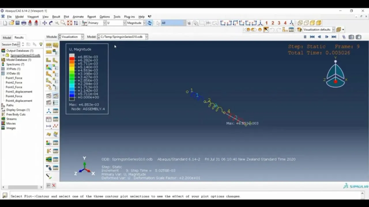


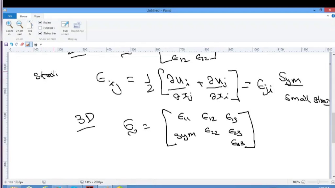

















Multi-step analysis in FEBio enables more realistic and stable finite element simulations by dividing complex loading scenarios into sequential phases; this approach addresses convergence issues with large deformations or hyperelastic materials by gradually applying loads (using time stepping and load controllers) and refining mesh resolution in critical regions (such as near fixed boundaries), ultimately producing accurate stress distributions and dynamic responses that would be difficult to achieve with single-step analyses.
FEBio Multi-Step Structural Analysis Tutorial
Added:Fundamental concepts of Finite Element Analysis (FEA), including mesh generation, node definition, and element types.
Basic principles of continuum mechanics, specifically stress, strain, constitutive relations, and boundary conditions.
Familiarity with the FEBio user interface (FEBioStudio) and the setup of basic, single-step static structural simulations.
An understanding of numerical solution methods, particularly Newton-Raphson iteration and basic time-integration schemes.
Advanced nonlinear material modeling in FEBio, such as hyperelastic, viscoelastic, and anisotropic material formulations.
Coupled multiphysics analysis, including biphasic (solid-fluid) mechanics and solute transport simulations.
Implementation of custom user materials and advanced boundary conditions using FEBio plugins or scripting.
Parameter optimization and material characterization using FEBio's optimization module (FEBioOpt) to match experimental data.
489 views19likes21:15Original Release: 2025-02-27
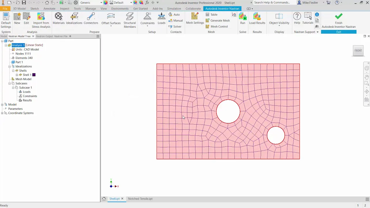
hello and welcome to this tutorial today we'll be discussing how to perform a multi-step analysis in fubio really it's just the tutorial from the website from the knowledge Suite here on fub bio.org but I figured that a video would be easier to follow than this text first off though why would we want to perform a multi-step analysis basically it comes down to kind of two things uh first making it as realistic as possible for example in my research we use these cervical spine models and if the nucleus pooses inside each of the discs isn't at the right pressure then the biomechanics don't like solve correctly and so we use one step to ramp up the pressure and then in the next step that is when we do all of our like loading and all our real analysis the second reason is for example um if you have like two contact surfaces and they're complex you may want to slowly bring them together before you do any like crazy motions so that they don't accidentally uh go through each other because the computer doesn't PCH them these multi-step analyses can kind of be a workaround to solve issues like that with that let's get started I'll open up a new window of Fe bio Studio here it is we're going to do a new model and it will be a structural mechanics type problem we're going to build our geometry we'll do this box and position 0000 0 that's perfect and we're going to give this a width of 10 units a height of one and a depth of 0.2 units so in X Direction 10 long one point2 these can be whatever units you need um in my research typically we use millimeters but you just have to make sure that whatever you decide on that the scales match between your different parameters so um I'm going to say 10 mm here for the width and we'll see that that affects how we Define our material later on so I clicked create and now here it is looks pretty good let's make a mesh we're going to come in here the object is selected and we're going to say since it's longest in the X direction we're going to give it the most elements in that direction so NX will be 20 n y will say five and then Z will say three now if I go ahead and apply this there's our stats that's how many we have and we can see that it created this beautiful mesh everything looks great um they're also all exactly the same size and shape which is great if we had everything else uniform along the material but actually we don't we're going to fix this left side and we're going to um apply a force on the right side and just from experience we know that um the stresses are higher closest to the fixed end and so to get better detail and a a more accurate picture of what's happening what we're going to do is apply an X bias so we're going to say x bias of 1.2 and apply there's our stats and so now we have the same number of elements as before but we can see that their shape has changed so This 1.2 means that if we take the length in X of this element to get the length in X of the next one over we have to multiply this length by 1.2 and so that compounds and gets bigger and bigger and bigger um which is exactly what we need for this case we also could do an X mirrored bias and so that would make it so that it was TI finer at both ends um we could do like um8 and that would do the same thing but backwards so we can hit apply and now it just fli it to the other side because it's the same thing this length by 08 by 08 by 08 right so we're going to leave it though at point2 and these are hex8 elements which means they're hexahedrons or cuboids and they have eight nodes each so in this case eight nodes hexahedron that means there's one at Each corner of the cuboid so anyways this is all all we need to do with our measure was these four things and apply so there we go it's all ready to go now now that's done let's come into our model viewer our steps this is where we're going to make our two steps our first step will um have a load and then our second step will let the load go and so it will bounce we haven't made those yet but there's actually already a step within steps it's called this initial step and this is kind of our base zero which what this initial step does is it gathers all the things that will be um applied during the entire analysis so every you know material definition boundary condition Etc that is on during the whole analysis starts in initial but then everything else we have to add an analysis step so you can rightclick and hit analysis step you can also come into physics add analysis step right there we want to insert it after initial there isn't really any other option anyway and so in this first step we are going to apply a load and we're going to pretend that it's static static means it doesn't move right and so it's going to be this quasistatic analysis meaning it just uses the like static kind of equations to solve everything so we're going to leave this analysis as static we're going to give this five time steps of length 0.2 so what does this time stepping do in the similar way that we had finer spatial resolution with our more refined mesh on this left Edge um the time stepping um Alters our temporal or Tim related resolution so if we rewind to classical finite element analysis everything is put in all at once and then in one step it says okay you had this you applied all these loads and boom you get this and it solves it all at once that's really hard to do with large deformations or hyperelastic materials like we frequently deal with in the body and biomechanics in general and so to counteract the issues that come with trying to go all at once such as you know maybe it accidentally calculates that things are like bumping inside of each other or themselves things like that to get around that we grab gradually add our loads at different time steps and so in this step we're going to have five time steps so broken down into five chunks and they're going to be 0.2 seconds long so 5 * 02 gives us one 1 second in our simulation time another thing we're going to do we're going to scroll down here and we're going to turn off the auto time stepper what does the auto time stepper do so when we apply our loads and let's say it goes one step in and it kind of runs into an issue then there are a number of things it can do to say okay maybe that step was too large let's work it back a little bit and so we'll add steps or decrease the time scale things like that as needed so that it can make it safely to that final point for this step we are confident that our five steps will be totally enough so we're just going to turn this off however we're going to leave that on for our other top Stu let's get that started so again right click add analysis step and we're adding this one after step one this will be step two and this is the one that we're going to make Dynamic we're going to make it 40 time steps long at 1 second intervals so this means okay 40 * 1 40 seconds plus our previous time steps so which was 1 second so we have 41 second simulation in all and all this we're going to leave this on um this is fine in the models that I work with we really get into you know probably 10 or 15 retries um changing the maximum and minimum step size turning on aggressiveness and things like that um to really help it get through the difficult parts of its solving but right now we can just leave that as is okay so that's our time steps let's come in and add our boundary conditions so we can come to boundary conditions right click we can also come to physics and add nodal boundary condition so this is how we're fixing the left side is we're adding a nodal Z displacement boundary condition so we'll hit okay and we're going to fix it in the X and the Y and the Z directions if you don't include all three then it might try to like shift a little bit in a certain direction but without any real guidance on how much or how little it's allowed to shift in that direction it will get really angry and it will either take a super long time or give you bizarre results or just crash and so we want to make sure that that it knows exactly how to move in all directions so we're going to fix in all directions here on this side so there it is and we want this to be part of the initial time step because we want this on the whole time and we're going to scroll down it's all set up except for we have to tell it which face to apply it to so we're going to do our select faces select this one and add add surface 4 to our zero displacement one boundary condition excellent I'm clicking off of that so that now it can come to the other side and we're going to add another one this time though it's not going to be a nodal boundary condition oh yeah it's going to [Music] be a surface load which there it is hard to find sometimes surface load and we're going to make this a traction we could have done noal we could have done a pressure things like that but the beauty of a surface load traction is that it will be the same no matter the area or the number of nodes of the surface it will just give this many newtons of force applied across the entire surface and so this one we want to be not part of the initial time step because we don't want it on the whole time we want it to be just with step one so that first second here's our scale what this does is it is a multiplication factor or the traction Vector right here so in here we have zero for X zero for y zero for Z we're going to move it or push it one Newton in the negative Z Direction so we're going to say minus one in that and then our scale is a multiplication Factor and this little symbol next to it shows that there's a load controller associated with it so to look at that we're not going to change it but just to look at it we can come up here to our curve editor and just like in our model viewer we have loads so loads we're going to drop down the menu traction one okay traction one and then inside traction one there's scale so just like how inside traction one there's scale there's scale inside Direction one and here's the load controller lc1 we have her over here oh if we hover over here we can see that it will tell us the name lc1 is our load controller I'll come right back and so as I said before this is how it ramps up the load over that 1 second so on our x axis we have time on our y- axis we have the scale so from 0 to 1 second it ramps up linearly and we can change this we can say okay make it a step smooth Etc um and we could say actually I don't want it to be negative one I want you to multiply it and make it 1.4 in the end or whatever we want to leave it at one for this I also want to make the point that we could totally use the load controller and not use extra steps so if I were to add I'm holding shift and clicking that adds a point and we could drop this down I'm can use this magnet so that it snaps we could have it ramp up and then turn off using the load control um and that would do the same thing as having this load only be part of step one and adding another step for later but um using the steps like in the tutorial um allows it to be easier like followed you know someone can come in and say okay this step happens this step happens instead of going something turned off oh it was in the load controller but that's just um multiple options so I'm going to select this and delete and so back to normal there we go so didn't really change anything can exit out and so we have the surface selected excellent and that's it it's part of step one so we're set our boundary conditions are ready to go and so now all that's left is adding material you can do that either by right clicking here or come to physics add material and I'm just going to search for Neo hooken so this is essentially the most simple material type in F bio so we're going to say 25,000 for Young's modulus ratio. 35 the poison ratio doesn't have units this is just the ratio of how much it like shrinks in as you stretch it and the Young's modulus though this one does have units so in our millimeters Newtons seconds scale that I like to use a value of 25,000 Newtons per millimeter squared that turns into 25 gigap pascals so 25 gigap pascals 354 ratio this is some sort of like a copper nickel alloy or something some sort of metal like that is what this would kind of represent um so that's our parameter values but we haven't added it to anything so I'm going to select the part there we can see the white bracket so it's selected now and just hit plus it turned orange so we know it applied and we're ready to go so I'll hit contrl s to save the FS2 file which is the F bio Studio to file so that saves all of the settings everything in um f bio studio and so I'll just save that to my desktop and I'll just leave it as model one you can rename it whatever you want okay that's good to go and now we're going to run it so we can click here Run f bio or come to F bio run so we click here and now it's asking what am I going to name the files that it uses to to run and actually process what we set up in here so this is going to make a fbio file or Feb which is different from the FS2 file that we just made the Feb file is an XML file sort of like a text file um and it has just everything listed in a giant like sheet and you can go in and you can edit parameters in there but that's what actually goes to the solver it also will create create a log file where it shows um all the stats and all the information from as it was running as it was solving and then it will also create axlt file or xlot which is the output file that will be reading in here in a second and so you can rename all those that'll all have the same name you can rename that here and uh you can see that it's going to save it to my desktop and then jobs so it's making a folder a jobs folder inside my desktop to put all that all right so no need to change any of that you can just hit run we can see in the upper leftand corner it's progress okay so we have our job monitor we have a normal termination uh it made it all the way to 100% so we're set I'd like to talk about These Warnings there are some warnings said the max number of iterations was reached so the stiffness Matrix was reformed basically um it did have a little bit of trouble as it was moving through those time steps but it was totally fine and it fixed it so warnings but no errors we're chilling so we'll open results and here it is I'm going to close notes and output so that we can look at the Timeline so I'm going to use my arrow keys to click through we can see the force is ramping up just like we set up in our load controller um up until time equals 1 and then from here it's going to release and we'll see the dynamic response and so there it is and you can see it kind of wobble and flop that's because the dynamic analysis includes things like inertia and density and mass and things like that and so there it is we can also come up here and look at stress for example effective stress you can see ah yes there the highest stresses are at the base and so it's a good thing we increased our spatial resolution with our finer mesh right there can also look at for example displacement say okay how high up does it go how low Etc and so we can see this is the Max height this is the minimum height and we can change some of this by selecting color map over here and yeah I recommend you play around with some of these parameters to see how it changes but that wraps up our tutorial thank you so much
Up Next

88:59
The Future of SEO: AI, Diversification, and Entrepreneurial Mindset
@SaketWahi
1.1K views•2025-02-20

12:54
Triumph of Orthodoxy Icon: Byzantine Art & History Explained
@BenCallan
2.1K views•2024-08-06

9:49
FastAPI vs Flask vs Django: Choosing the Right Python Web Framework
@TechWithTim
302.5K views•2024-05-26

1:42
Game of Thrones Opening Credits: A Cinematic Analysis
@gameofthrones
46.3M views•2011-04-18
Related Study Plans & Knowledge Roadmaps
Structured learning paths in General & Interdisciplinary Studies
general-studies
Elevator Engineering: History, Physics & Cities
01From Hoists to Safety Brakes: The Dawn of Vertical Lift
02Hydraulic vs. Traction: The Engineering Physics of Elevators
03Modern Speed, Safety, and Algorithms
+ 2 more learning modules
12h5 modules
Explore Roadmap
general-studies
Rubber: Material Science, History & Geopolitics
01Origins of Natural Rubber & Mesoamerican History
02The Chemistry of Natural Rubber & Vulcanization
03The Geopolitics of the Rubber Boom & Colonization
+ 2 more learning modules
12h5 modules
Explore Roadmap
general-studies
Containerization: Evolution, Logistics & Trade
01Ancient Trade & Bulk Cargo: Amphorae to Barrels
02The Industrial Revolution & Cardboard Packaging
03The Containerization Revolution: Malcom McLean
+ 2 more learning modules
12h5 modules
Explore Roadmap
general-studies
Textile Tech: Evolution, Labor & Global Impact
01Pre-Industrial Textiles: Handloom & Cottage Industry
02Mechanization: The Spinning Jenny to the Power Loom
03The Factory System & Global Labor Transformation
+ 2 more learning modules
10h5 modules
Explore Roadmap