



















The IS-LM model combines the goods market (IS curve) and money market (LM curve) to determine equilibrium income and interest rates; the IS curve shows the negative relationship between interest rates and income through investment responsiveness, while the LM curve reflects money demand and supply dynamics, with monetary policy effectiveness varying across the business cycle due to changing investment sensitivity to interest rates.
IS-LM Model: Goods & Money Market Equilibrium Explained | Economics 313
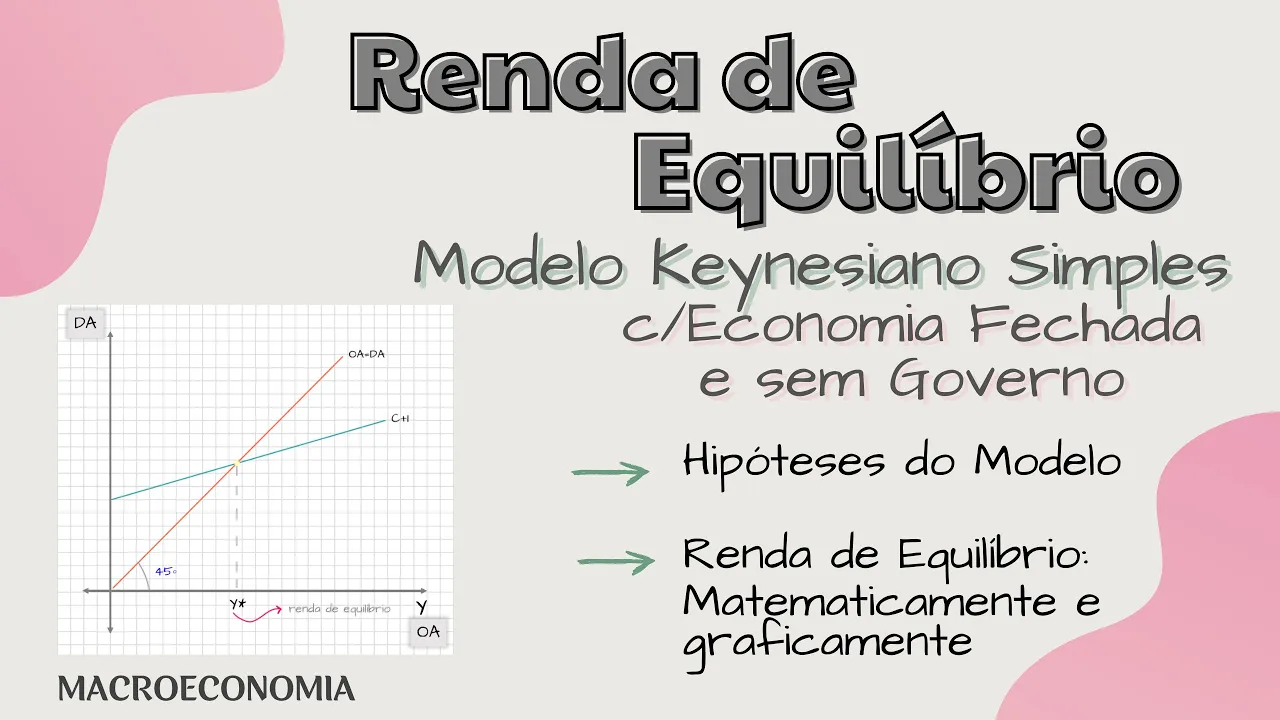
Added:The Keynesian Cross model and the determination of equilibrium output in the goods market.
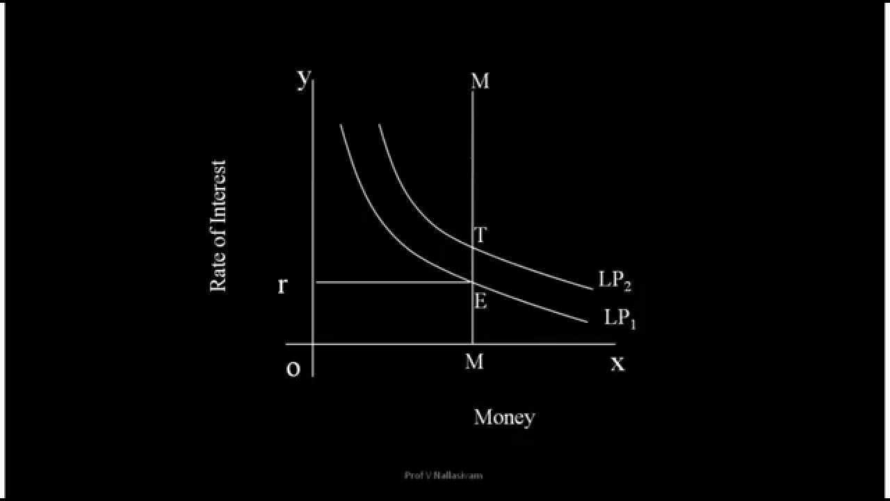
Liquidity Preference Theory and how demand and supply of money determine equilibrium interest rates.
The fundamental components of aggregate demand, particularly the relationship between interest rates and investment.
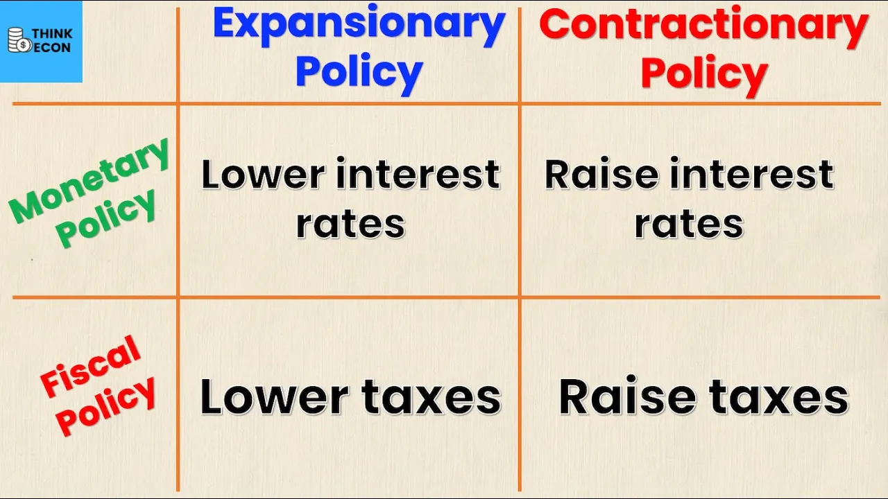
Basic mechanisms of fiscal policy (government spending and taxation) and monetary policy (money supply adjustments by central banks).
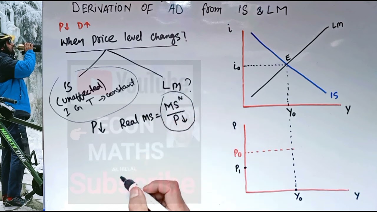
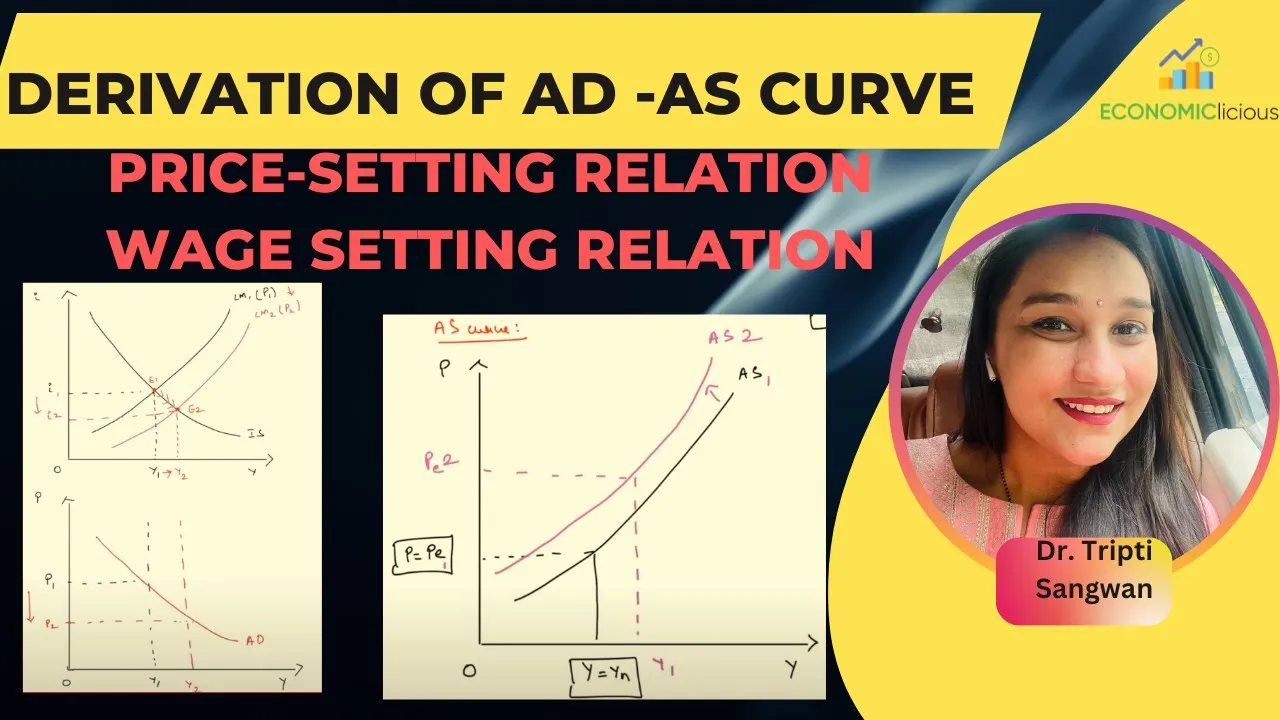
Derivation of the Aggregate Demand (AD) curve from the IS-LM equilibrium and the transition to the full AD-AS (Aggregate Demand-Aggregate Supply) model.
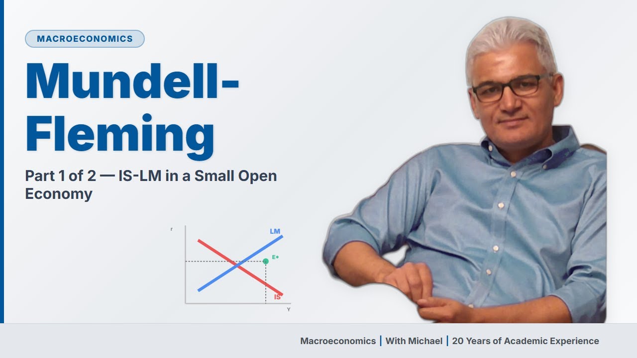
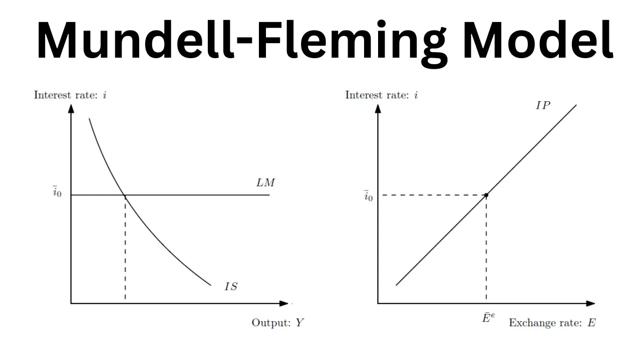
The Mundell-Fleming Model, which extends the IS-LM framework to open economies with trade and capital mobility.
Analysis of policy extremes, including the liquidity trap, the crowding-out effect, and the zero lower bound.
The transition to modern microfounded macroeconomic models, such as New Keynesian Dynamic Stochastic General Equilibrium (DSGE) models.
4.3K views56likes1:28:24Original Release: 2017-01-14
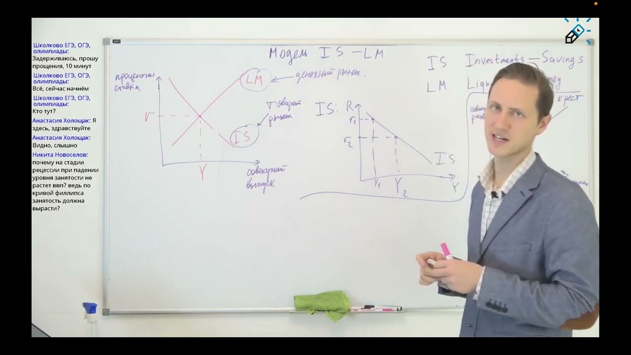
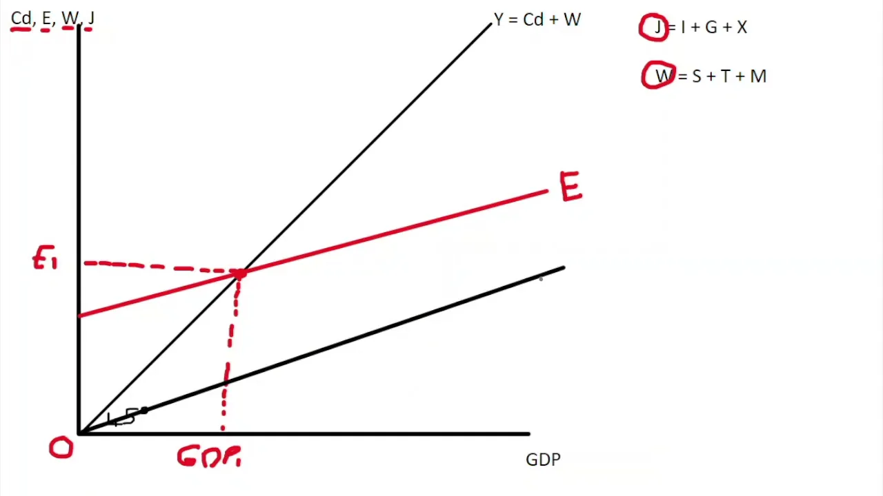
hello again in this video we're going to cover chapter five on the is and LM curves you might notice I look a little different than the other videos that's because in the latest edition of the book the seventh edition they've changed this chapter quite a bit and so have to redo the video to reflect that there's another implication though if you're using a previous edition of the textbook say the sixth or earlier this chapter is going to be quite a bit different the another chapter we're going to cover chapter nine is not even in the old book at all it's replaced another chapter and it's written in a completely different way and they've reordered the the numbering a little bit so if you're using a previous edition of the book it's probably not going to work very well from here on out so just thought I'd let you know that okay in this video what we're going to do is put the Goods Market and the money market together so we've talked about the goods market in terms of the 45 degree line diagram looked at the money demand money supply curves we're going to take the Goods Market Drive something called an is curve we'll take the money market Drive something called an LM curve then we can put them together and together we can find that one unique point it's going to turn out to be a combination of the interest rate and income that gives us an overall economy WI equilibrium it's an equilibrium in both of those markets at the same time so that that's where we're headed and you'll see how it works as as we go along here so let's um start with the goods market now up to this point our model of the Goods Market has been something like well not something like it has been y equals c of disposable income consumption plus I plus G bar so consumption dependent on disposable income both investment and government spending were assumed to be completely exogenous now for invest for government spending that's a decent assumption for investment that was a simplifying assumption and we're going to need to fix that at this point so what we're going to say now is that investment is some function of the interest rate in income and we're going to assume that as the interest rate goes up investment goes down there's a negative relationship so when R goes up investment goes down for those of you whove had calculus what we're saying is the partial of I with respect to R is less than zero and for income we're going to say when income goes up when GDP goes up investment tends to go up so I of Y the partial of I with respect to Y is going to be greater than zero this this I ofr parameter this relationship between the interest rate and income will play a big role later and we we'll come to that um okay now let me explain this a little more why is this negative and why is this a positive relationship so let's talk about the relationship between investment and income first so let's just think of a single firm all firms would be doing something similar um let's let's take and look at a bunch of potential investment projects and let's just arbitrarily name them A B C D and E and each one of these projects will have an expected rate of return on the investment so let's say this first one's really good project you think so you expect 14% this one's not as great but still pretty good 11% get to see we're falling down to 6% 4% 2% for e and so we've got these ordered in terms of their expected rates of return we can also just m I'm just making up these numbers but let's just do some costs maybe this first one's a million dollars maybe the second one 2 million third one four $400,000 fourth one I don't know million and a half and the last one 3 million so then the question is how many of these projects should the firm undertake so let's assume that the interest rate to begin with is 12% pretty high interest rate but it'll work for an example at a 12% rate of interest project a would be worthwhile because you're going to earn 14% on your million doll investment it's going to cost you 12% to borrow the money or even if it's your own money retained earnings you could lend it out at 12% because that's the interest rate so that's your opportunity cost that's what's going to cost you to invest in this project so you're going to make a 2% net rate of return but when you get to Project B you're only going you're you're not going to want to invest because you're going to have a negative 1% expected um revenues minus costs so in this case only investment a would be undertaken so investment would be a million dollar now suppose that the interest rate Falls to let's say 8% well now Project B is going to also pay but C won't so now your investment would be a plus b so your total investment would go from1 million to $3 million and we can imagine all the firms all across the country doing this so as the interest rate Falls more and more investment projects become viable become expected profitable and you'll get more and more investment and you can see if the interest rate kept falling to say 5% then your investment will be 3,400,000 if it falls to 3% you're going to invest in D and if it somehow fell to 1% you you'd also invest in E so as that interest rate goes down more and more investment projects become profitable and investment tends to go up so that's really all there is to the relationship between the interest rate and investment as the interest rate goes down it's less costly to borrow money so you tend to see more investment for income it's it's a fairly easy um thing as well we just think that well as income goes up um as GDP goes up firms are going to be more confident about the future they could be running into capacity problems they need to expand and because GDP is growing their customer base their sales are growing that sort of thing so as GDP goes up we tend to see more investment and so so that's all the is so our model is going to be y equals c of Yus t plus I of R and Y plus G and I I won't always remember to put the bar on G but we'll just understand that that is an exogenous variable now our goal here to to derive this thing called the is curve is to work out the relationship between interest rate and income if I change the interest rate how does income have to change to keep this in equality okay now we've already drawn a picture of this what we did was put income on this axis we put they called it Z in the book but it's aggregate demand this thing that's demand Z is demand and we noted that you can you can model this as a 45 degree line diagram and then put this function C + I + G and then where that intersects gives us our level of income now what we want to do is is is work out how income if I change the interest rate the interest rates in this function I of R and Y there's also a y minus t in there but I don't need it if I change that R how does income change at equilibrium so if I call this initial interest rate r0 that's supposed to be a comma there if I let the interest rate go down to R1 what's going to happen well investment's going to go up right so investment will go up you'll have C plus I of R1 y + G where R1 is less than r0 and so what's going to happen is income will go up so when we when R goes down income goes up so it looks like there's a negative relationship between the interest rate and income so let's do this a little more systematically we can actually derive this thing called the is curve graphically what we're going to need are two different graphs so we're going to need a 45 degree line and down here we'll keep track of the relationship between the interest rate and income so this was income Z aggregate demand we have the 45 degree line diagram and let's call this C+ I of r0 plus G I'm just dropping the other Arguments for clarity so at an interest rate of r0 income is y0 so let's come down here here's y z and let's just r0 is somewhere on here let's just say it's right there okay so that's our initial equilibrium point in the Goods Market so this is the Goods Market that's one pair R and Y that's an equilibrium now what we want to do is draw the interest rate to R1 and see what happens well if we drop the interest rate to R1 this is going to shift up to C + I of R1 + G not a very good R1 there and now income goes up to y1 so at an interest rate of R1 income is y1 now we could keep doing this I could pick interest right here or here let's just pick one even a little lower R2 D2 so at R2 this is going to go up again C + I of R2 + G keep forgetting that parentheses Ah that's pretty messy C + i r R1 + G C + I of R2 + G we make sure that's on the screen yep and so now at R2 income goes up to Y2 find that point down here so here's R2 and Y2 so you can see we're starting to map out a curve if I were to pick every possible interest rate it would show me every possible income and what would happen is I would map out some curve and we're going to call that the is curve so the is curve just keeps track of all the equilibrium pairs r0 y0 R1 y1 R2 Y2 all the equilibrium pairs in the Goods Market so it's every possible combination R and Y that's an equilibrium in the Goods Market now why is it called the is curve is stands for investment equals saving and we're using an income equals expenditures approach so we're using Y = C + I + G this side is expenditures this side is income and so yal e is our equilibrium but you can also write income as consumption plus savings plus taxes that's all the uses of your income right they take taxes out of your paycheck you take it home you either consume it or save it okay so what we can do is cross out those C's they cancel so s + t = i + G this is what we call voluntary savings that's the savings you want to make this is force Savings in some sense this is the amount the government makes you save out of your paycheck for things like Social Security or it takes it and spends it but it takes it you can think of it as savings this is this similar here this is private investment and this is government investment so alt together we have savings both private and public equals investment which is both private and public or if the budget's in Balance which in the 1930s when they first started using these models it wasn't unheard of for t equal to G it's a little bit range for us these days and in that case s equals I so our equilibrium is is yals e I don't think you can see that up there can you oh maybe so so our equilibrium is income equals expenditures but mathematically it's equivalent to savings equals investment in in in a more general term so the is curve is just investment equals savings it's just a way of saying it's the goods market equilibrium okay let's do shifts in the is curve next make sure I got everything I wanted to say looks like it so what we need to figure out is what makes the is curve shift in or shift out and really it's pretty simple anything that causes aggregate demand to go up except a change in the interest rate when you move along the is curve anything else that causes demand to go up will cause the is curve to shift out so let's do a couple of examples of that so we're going to show this graphically so we're going to we're going to show how the is curve shifts with these double graph models so down here we have the is curve R and Y here's the 45° line diagram and I'm going to use government spending as my first example but you'll see that so I'm going to call this C+ I + g0 you'll see it's the same for for other things as well so here's y0 now let's assume we've already derived the is curve and let's just find this equilibrium point which is y z and r0 so in in I here there's an r0o it's I of R Zer now if we let government spending go up so what we're going to do is we're going to let government spending go go up holding R constant and that's important so maybe I should actually highlight that sorry about this for your notes this is I of r0 plus g0 so we're at r0 y0 and g0 we're going to increase government spinning but we're going to keep r at r0 all right so let's do that we already know how this H what happens here we we've done this before when government spending goes up this will shift to C plus I still at r0 plus G1 and so now we're income level of y1 but the interest rate is r0 so we're at that point now this is an equilibrium in the Goods Market so it has to be on the is curve so that tells us that the is curve must have shifted from from is of g0 Z to is is not I is of G1 so when government spending goes up the is curve shifts out now notice that this shift would have been the same if I had cut taxes if there had been an increase in consumer comp confidence an increase in business confidence anything that shifts this up except a change in the interest rate which would move us from there to there anything that shifts this up other than a change in the interest rate is going to cause the is curve to shift out so if we wanted to do taxes all we'd have to do is just relabel these let's let's do a tax cut instead well it's exactly the same except you have C of y - t0 + I of r0 plus G and this one taxes went down so shifts up C of Yus T1 + I of r0 + G so again it's exactly the same we cut taxes this curve shifts up shifts the is curve out this is t0 this is T1 T1 let than t0 if we had done consumer confidence same thing confidence went up this would shift up business confidence shifts up so you get the idea anything that shifts the 45 degree line up and we went all through that earlier in the course will cause the is curve to shift out the four main things that we're going to use in the in the quizzes and in the class are government spending taxes business business confidence and consumer confidence so G up T down confidence up this will shift up shifts the is curve out and the opposite of course would shift the is curve in if this had been t0 and this had been T1 and taxes had gone up we would shift back the other way and so it's it works in both directions so that's the is curve terms of how to drive it and what makes it shift and we'll be using some examples of that once we get the LM curve in let's do a little bit on the slope of the is curve now I'm not going to ask you to do this but let me do it mathematically first so that those of you who follow this can can see that it's really easy to see when you do it mathematically what's going on here so let's say y our our model is y = c of y - t + I of R and Y plus G we want to find the slope of the is curve so there's Y and R so we want Dr Dy that would be the slope so what I need to do is take take a total derivative so if you hopefully you've had multivariate calculus or they talked about it regular calculus and then we'll solve for Dr Dy so we we're going to totally differentiate this Dy is the partial of C with respect to Yus T C of Yus T * Dy minus DT plus I of r Dr R plus I of Y Dy plus d g so that's what's called the total derivative of that function now we want Dr Dy all else equal and so we're going to hold tax's constant so DT is zero we're going to hold government spending constant so DG is zero so now we have Dy is C of Yus T Dy plus I of r d r plus I of Y Dy so Dy * 1 - c of y - t - I of y = i of R Dr R so now we have our answer Dr Dy I is 1 - c of y - t - I of Y over I of R so that's the slope so you can see that if consumption goes up this will be a smaller number it'll get flatter if I of Y goes up same thing this will be flatter we generally assume by the way that c of Yus t plus I of Y is less than one you run into some problems in the model if that's not true so when these things go up they get closer to one this gets closer to zero and um the slope Falls now I of R is a negative number but when it goes up in magnitude like from minus1 to minus 20 that's actually smaller but it's bigger in magnitude when this so when this gets bigger in magnitude the slope gets flatter so the bigger I of R is the flatter the Curve will be and that's going to be important later so I'm going to show that graphically I'm going to look at the relation how the slope of the is curve changes when I of R the responsiveness of investment to interest rate this is how investment changes when the interest rate changes we're going to look at how the slope of the is curve changes when I of R changes so what I'm going to do is simultaneously derive the is curve twice under two different assumptions a small in magnitude I of r or a big absolute value of I of R so we knowed to derve it we need this 45 degree line put together with this Y and R graph so this is z I'd prefer to call this e for expenditures but the book calls it Z can't help that there's y so let's start off with with um here's our 45 degree line and here's C plus I of r0 plus G so our starting point is this point y0 and r0 now we're going to let R go down and we're going to have two different I assumptions about I of r one that it's tiny in magnitude one that it's big in magnitude and then we're going to see how the curve changes so let's set R go down to R1 here okay what that parameter does when R goes down this shifts up and the reason it shifts up is because investment goes up so if I of R were relatively small if the response of investment to the interest rate is relatively small this isn't going to shift up very far and so in that case it might only shift up to to C plus I of R1 plus G and this is for I'm going to use absolute value because it's a negative number and I'm I'm talking about the magnitude I of R is small so it doesn't shift up very far so in that case our is curve would look like that now we can think of a second case where I of R is a whole lot bigger if I of R is bigger for a for the same fall in the interest rate investment's going to go up more and so in that case might be this C + I of R1 + G and this is for I of R larger than it was here so because it's larger we get a bigger shift right so there's y 1 Prime so in that case we'd be there so that would be our point in the is curve and we can see that the is curve gets flatter and so our result is that as I of R and just we're going to use a word for this this is how responsive investment is at the interest rate when it gets more responsive when a given fall in the interest rate gives you a bigger change in investment that's going to cause the is curve to get flatter and if you go back and look at that that slope formula 1 minus C of y - t + I of Y over I of R that's Dr DY for the is curve you can see that as this gets go as this gets to be a bigger number this is going to be you're going to get a smaller slope a flatter a flatter curve and so I of R going up flattens the is curve now now why am I spending so much time with with what seems like a just a technical detail about the slope of the is curve well this I ofr really varies a lot over the business cycle so when you're at near full employment investment tends to be fairly responsive to the interest rate because you're already at capacity interest rate Falls you want to expand it's a good time to do it business is good you tend to see a lot of investment in deep recessions you tend to see less responsiveness of investment to the interest rate and the reason is that you know think of the Great Recession firms had idle factories they have half their trucks or delivery trucks might be sitting in the lot maybe you're a restaurant and half your tables aren't being used why would a small fall in the interest rate cause you to do any investment when you already have all this excess capacity so there's really very little reason to invest and plus you're looking forward and thinking gez I don't know when things are going to get better why should I take a risk now spending a lot of money on investment when aggregate demand may be down low like it is now for quite a bit of time so you don't tend to see much responsiveness to the interest rate when you're in a recession near full employment you might be thinking oh gosh my restaurant's full I'm you know my factory is full I I'm running out of trucks to do delivery but boy I at the interest rate as high as it is right now it's just not quite worth it to expand but the minute that falls they'll be say oh now it's worth it you know we went from Project a to Project B in our earlier example and now you'll see lots of firms investing so you see a lot more responsiveness near full employment than than in recessions and that's going to have a big impact on the on the ability of monetary policy to stimulate the economy as we'll see later and so this parameter I ofr changing this the responsiveness of investment interest rate changing has important implications for whether we should use monetary or fiscal policy in a recession and that's something I'll come back to in a few moments excuse me for a sec okay so I think that pretty much does it for the is curve let's turn to the LM curve now we've already looked at a model of the money market said okay you can put M on this axis the interest rate on this axis and we had a a a money supply curve and a money demand curve py L of I and this L standed stood for liquidity preference the the term LM L usually stands for money demand because it's an old term from K's for liquidity preference which is the way he talked about it I think we talked about that earlier and then m is just for the money supply so what LM means is simply money demand equals money supply so the LM curve is going to be just like the is curve was all the points where where where demand expenditures equals income essentially Supply equals demand this is the same thing it's where money demand equals money supply alrighty now we're going to change this just slightly because it makes something we're going to do in a moment easier let me let me let me show you what we're going to do our model is we say well money supply equals m money demand equals p y l of I so money Supply equals money demand is m equals p y l of I and that's what that diagram is showing is this is the the downward slopping line and this is the vertical line because we assume the FED can control the money supply perfectly it's a little more convenient to just divide by P call this real money money divided by the price level that's the purchasing power of a dollar is equal to y l of I this is real money demand one way to think of this this is money demand a lot of it's carried around for transactions so what this is really saying is that this is the amount of stuff you buy in real terms like like the number of oranges or the number of bicycles and so on although it so if you hold that constant if you double prices you're gonna have to double the amount of income that you carry to buy the same amount of stuff so if we hold this side constant just double prices that's going to double m and what it's saying is if if if you're going to buy the same amount of stuff and prices are twice as high as they were before you should carry twice as much money and so this is just stating money demand equals money supply in real terms now graphically it's not a whole oh I'm using I here I is the same as R um most of the time I is equal to the nominal interest rate and R is equal to the real interest rate but we don't have any inflation yet which is the difference between the two because in the islm model I haven't really said this yet but the price level is held constant so Y and R vary but the price is assumed constant and so um can't remember the point of was going to make ah oh and so in this case I is equal to R usually the nominal interest rate is the real interest rate plus the expected inflation rate but this is zero for us right now very soon like by chapter nine for sure but even sooner than that next chapter actually um that assumption will be dropped and we'll have to distinguish between the real and the nominal interest rates so I've been slipping between I and R and I I apologize for that but it doesn't really matter as long as you understand all righty so um let's derive the LM curve just like before because at this time we have to put the the graph side by side I'll explain why so we want to dve this thing called the LM curve so we want the relationship between income and the interest rate and we're going to use this real money demand money supply diagram to work that out so this is going to be M over P we divide it through by P and this term here is going to be um y l I'm going to call this y0 L of I so that gives us r0 so we could last time the two graphs shared the the horizontal axis this was y in the Goods Market so we stack them vertically this time they they they share this axis so we put them side by side so the axes line up so I can come over here and figure out okay here's r0 and just pick one it's somewhere let's say it's there there's y zero now we want to know what happens if income goes up what happens if income goes up we know that's going to increase money demand and so what'll happen is you'll go to y1 L of i l of r I'm so used to using r i so at R1 at y1 the interp would rise to R1 and so we can come over here now I could pick a bunch more levels of income may maybe this one and map out other points but when we're all done we'll get this relationship called the LM curve and what the LM curve is is it's all of the combinations of Y and R that are in equilibrium there's one equilibrium there's another another pair of R and Y that's an equilibrium so it's every pair R and Y that's an equilibrium in the money market before going on I'm going to backtrack momentarily because there's something I forgot to say about the slope of the is curve that I meant to do so that's how you drive the LM curve we need to look at shifts in the LM curve then I need to point out that this is not quite how the book does it and then I'll I'll I'll reconcile the two for you okay but let me backtrack for just a second I did the slope of the is curve graphically mathematically I forgot to do an intuitively so what's what's the intuition so if you if you look at the is curve what's going on so here here's here's r0 and Y Z y1 and R1 what's going on here is that as we lower the interest rate investment goes up and this is where that I of R parameter comes into play I of R tells you that for a given R fall how much investment goes up then income goes up and this is by the the multiplier so the multiplier plays a role here we're holding that constant and I of R comes in here so in this case we lowered the interest rate investment went up and that drove income up now if I of R had been even bigger what would happen so this is the the the first case now let I of R be bigger in magnitude so if I of R goes up you'll get a larger change larger change triangle is change change in y for a given fall in R so if I of R had been bigger for a given say from 10% to 4% investment goes up even more so income goes up even more so if I of R had been larger we would have gotten a bigger change and the is curve would be even flatter and so as I of R goes up you get a bigger change in y for a given Fallen R the bigger the change in y the flatter the is curve so that that's the intuition for the slope of the is curve and sorry to have to backtrack back like that so let's let's get back on back on track too many tracks all right um so we've derived the LM curve let's do shifts in the LM curve so what's going to make the LM curve shift the main thing I want to focus on is a change in the money supply so let's let's do that so we've got our real money supply M over p real money demand y z l of I call this m0 up here so at m0 we are at r0 and y0 now let's assume the LM curve has already been derived its position's going to depend upon M over p and let's find the point we're at r0 y z so we're at that point now we're going to hold income constant y z change M and see what happens to R all righty so let's set M go up that's going to cause M over P to go up if we hold P constant so that's going to shift this out to M1 over P so that's going to cause the interest rate to fall income hasn't changed so now we're at that point right there well that's a combination R and Y that's in equilibrium it has to be on the LM curve since that's what the LM curve is is all those points so the LM curve must have shifted out same thing would happen by the way if I had just let the price level go down this would shift out as well so what matters for the LM curve is at M overp but what's important for us is when M goes up M over p goes up and that causes the is curve to to shift to the right to shift out some people get confused you could describe the shift two ways it either shifts down or it shifts out either one similarly if you go the other direction you can say it shifts up or in so those are equivalent statements out and down for the LM curve would be same thing so now we know how the LM curve shifts shifts out when there's a change in M or a fall in P there's other reasons it could shift too but that's only ones we're going to need now the book does the LM curve what it calls the LM curve is not what's traditionally called the LM curve and so let me now try to show you how to get from this is the traditional way to do the LM curve and the book does a different way entirely so let me try to connect the two somehow not somehow let me let me I will connect the to okay so let's now um put the is and the LM curves together so at this point traditionally what you do is now say okay we've got this thing called the is curve that's all the RS and Y's for the goods market we've got this thing called the LM curve which is all the RS and Y's for the money market that are equilibrium and so there's this one unique point right here y z and r0 that's an equilibrium in both markets then traditionally what you would do at this point is look at okay this this is curve depends upon government spending and taxes confidence other things this depends upon M overp and so we could say well if government spending goes up the is curve would shift and income would go up and the interest rate would go up or M change something would happen we're not going to do that because this this model assumes that the FED targets the money supply when in fact what the FED targets these days that was true a long time ago when they when they built this islm model assuming the FED targeted M was a good assumption but they don't do that anymore what they target is the interest rate and so we want to to somehow capture that in our model so traditionally monetary policy was viewed as a change in m so what you would do is say well the economy is in a recession we need to increase the money supply say to M1 over P hopefully that'll increase income and at the same time it ought to decrease the interest rate and so we view the FED as controlling this thing M but that's really not what they do today they actually control what they what they really control is something called the federal funds rate but it's essentially they control interest rates now let me back up for just a second and go back to the money demand money supply diagram and make a simple point that the FED can't control M and um r at the same time this should be M here r so what I'm trying to show you is that the FED has to make a choice between an interest rate target and a money Target the LM curve is derived under the assumption that they have a money Target so there's I'm going to go back to the nominal version of this so there's some Target for money M star and you've got this um py L ofi money demand and let's just say you're lucky and you have some interest rate target and you just happen to be at both to start off here so you're both at the interest rate target and the money Target and let's suppose there's some Shock some reason why maybe prices change or something else happens but for some reason this money demand curve shifts so say the price level goes up say there's an oil price shock or something what what something makes the price level go up well now suddenly we're no longer at our interest rate target but we're still at our money Target and so now we're only at one of our targets we we're not at both we could stay at our money Target or if we wanted to we could increase the money supply to get back to the interest rate target but you can't stay at both you have to make a choice and so the FED has to make a choice between do I want to keep the interest rate constant until I decide to change it to a new Target but do I want to Target the interest rate or do I want to Target the money supply the LM curve was built on the assumption that they targeted the money supply but that's not what they do these days as I've said they target the interest rate so when they target the money supply what happens is the interest rate adjusts you you can't control the interest rate so just to do the same examples as before you've got p y l of I some price shock you've got M Star start off at R star if you want to keep a money Target and there's these shocks the interest rate is the variable that adjusts so now we would go up here to R so we're going to keep the money fixing at M Star because we've got a money Target as the FED that that's our operating procedure we target the money supply well in that case m is exogenous it's determined by the fed and R is endogenous it's going to adjust to give you an equilibrium in the Goods Market it could be anywhere so R is the endogenous or the adjusting variable and M is the exogenous of the variable chosen by the fed the way it works now is that the that completely reverse now what the FED does is it targets an interest rate so here's m r m p I'll keep using the same example that price change so here's our interest rate target R star now when there's a disturbance like an increase in the price level to P1 y l of I what the FED does is it just lets the money do the adjusting so it'll it'll look out into markets and it'll say oh the interest rates above Target so it'll start engaging in open market operations and increasing the money supply and bringing the interest rate back down to Target so now what would happen is the interest the the money supply would adjust now the money supply is the endogenous or the adjusting variable and R is the chosen variable or the exogenous variable and so monetary policy is just a horizontal line at at r star okay let's go back to the islm so let's let's start off with it with interest rate targeted so last time the way we did monetary policy traditionally the way we thought about monetary policy is a Fed would manipulate this m to hit some goal but that's not how it works anymore what the FED does is they control the money supply so let's suppose that for some reason the is curve shifts out maybe there's a change in taxes or or business confidence changes something like that the is curve shifts out under a money Target you wouldn't do anything because you're still at M you would like R adjust to whatever the money Target is to you'd like R adjust to make equilibrium and now what happens is is the Fed has this money Target or interest rate target sorry so what it'll do is it'll increase the money supply it'll say oh the interest rate is too high excuse me in markets so what we need to do is increase the money supply to bring the economy back to our targeted level of of the interest rate and when all is said and done income would have gone up but now m is just adjusted to whatever it needs to be there is no money Target like in the old days M has just adjusted to whatever it needs to be in order to maintain the interest rate target so you're always going to end up along this horizontal line no matter what happens the Fed will adjust M to keep r at R star so what the book does is it just dispenses with the traditional LM curve all together and it writes the is LM curve as here's Y and R here's the is curve for the book The LM curve is just a horizontal line at the interest rate target because the fed's going to do whatever it needs to do to the money supply to make sure that we're at that interest rate target now I really don't like calling this an LM curve because traditionally the LM curve is an upward sloping curve that reflects a money Target in most places this would be called an M peer for monetary policy our policy is our star in this case sometimes s the policy is more complicated you get an upward sloping curve and it's it's usually called the MP or the monetary policy curve this book calls it the LM curve I don't want to confuse you by using two different names MP and LM for the same thing so I'm going to go ahead and call this the LM curve slightly under protest and so whenever um unless I really say otherwise and make it clear I'm talking about the old fash an LM curve when I use the term LM on exams or quizzes or review questions or or from here on we're going to mean the book's horizontal Ln curve and it's just shows that monetary policy is a fixed interest rate at that policy you would get y z the book of it doesn't have a star here and they just call this a policy rate and it's understood that that's the variable that the FED is controlling okay so now we finally have um our islm model as as the book does them now we need to go through um monetary and fiscal policy so let's start with fiscal policy monetary policiy going to be easy it's just going to be changes in the Target interest rate it'll move this line up or down fiscal policy is going to move the is curve around but let's go through it very quickly just so we can see how it works it's pretty simple I think hopefully for once we'll see okay so fiscal policy in the islm model nice why um all right so let's start off y r is I I could I'm going to use government spending we could ju an increase in government spending is going to look exactly like a decline in taxes or I could use business confidence or consumer confidence when they go up it's going to shift the is curve just like an increase in G so I'm using an increase in G but it's more General it's it's exactly the same as for a decline in taxes or an increase in confidence so anything that's going to shift this is curve so here's our Target I think the book calls this R Bar maybe even I bar let me look real quick make sure I'm using the right oh the book uses and I've been using R again they're the same ah oh well I and R are the same for now so the book calls this I the reason I was using R when we get to chapter nine this is suddenly going to flip to R in the book so the book's a bit inconsistent I was going to try to use R all the way through but I guess if I want to do the same thing the book does I better use an I um so iar is the fed's interest rate target at that Target we would get an output level of Y call it y zero now let's suppose there's an increase in government spending taxes go down this is the example I'll use confidence goes up so on that's going to shift the is curve out to is of G 1 and at G1 income would be y1 and so when government spending goes up that causes aggregate demand to go up and then that causes income to go up and so that's really all there is to it um you know I should have put LM here you probably don't want to write this down but in in the old days the LM curve would have looked like this and if the FED had and this would be LM of say m 0 over P what the FED then does is increase the money supply to LM of M1 over p in order to maintain their money Target and so in terms of our other model that's what would be going on government spending goes up that puts upward pressure on the interest rate the FED responds by loosening policy to keep the interest rate at its targeted level all right that's fiscal policy monetary policy let's do monetary policy next anything else I wanted to say there no this is equally easy here's Y and I finally got it right here's I bar zero that's their initial policy here's the is curve I'm not going to care put the arguments in because we're not going to change any of them here's I this is LM monetary policy is just a a new interest rate target so let's say the FED thinks that income's too low full employment's out here somewhere so what it'll do is they'll they'll meet and they'll say okay let's let's change the interest rate target to bar one let's lower the the Target and when they do that income will go up to y1 and so monetary policy is just the change in the interest rate so the outcome is that you get a higher level of income what goes on is that when when the interest rate goes down that causes investment to go up which causes income to go up that should look exactly like our discussion about the slope of the is curve because it is you moved from there to there that is the slope and you can see that how much Y is going to change for a given monetary policy is going to depend upon the slope of that is curve so that's what we're going to do next is policy Effectiveness you may want to draw a different graph I'll kind of pace around here for a second in case you want to that um or I iess you could hit pause button huh um I'm gonna do it the same dra if in a recession the responsiveness of investment to the interest rate goes down and the is gets steeper so the is curve tends to be steeper in recessions than it is at full employment so this might be the Full Employment picture this is how much output would go up because investment's fairly responsive in a recession this is curve might be steeper so this is the one for for I of R smaller in that case the change in income would only be to y1 Prime so instead of going all the way here to y1 you only go to y1 Prime so what does that tell you about the the effectiveness of monetary policy well it tells you that in recessions monetary policy is not as effective as it is at full employment and so at full employment monetary policy tends to be really effective it's really good at at slowing down the economy when when you're at full employment you T you see inflation the FED can jack up the interest rate that'll have a big effect on investment and and that'll have bring aggregate demand and inflation back down in a in a recession lowering the interest rate doesn't do much for investment for the reasons we talked about earlier there's already a lot of excess capacity why bother to invest and so in that case monetary policy loses its Effectiveness and so that's the first point so the the section we're doing right now is policy Effectiveness monetary policy Effectiveness so in a recession the responsiveness of investment responsiveness of I to r or I makes no difference Falls and that causes the is curve to be steeper and monetary policy is less effective and again just to redraw it quick there's the recession is curve there's the Full Employment is curve there's your initial interest rate i z initial level of income when we drop the interest rate to i1 Effectiveness means how much it impacts income in this case it's really small so there's the recession near full employment exactly the same policy gives you let's say near full employment the exact same policy gives you a much bigger change in income now there's actually a case where mon monary policy can become completely ineffective in a recession and this brings up something called the zero lower bound or sometimes called the liquidity trap let me show you this so here's y i here's our initial policy iar kn here's the is curve and let's just assume that monetary policy has been managed so that this is the natural rate with the book calls YN this is full employment the natural rate of output and then like in the Great Recession something happens that shifts this op S curve way back in fact so far back that it intersects the Y AIS at something less than YN so then the economy goes into this big recession what would the FED start doing well the fed's going to want to lower the interest rate right so the FED starts lowering the interest rate just like it did right in 2007 after the recession they were pretty aggressive iive um and bringing it down so they start bringing the interest rate down output begins going up but eventually they hit this zero lower bound this is zero and you can't have negative interest rates some people say you can that's irrelevant because the Fed was really unwilling to do it even if you could they were not going to push the interest rate below zero because they were worried about that's really Uncharted Territory we don't know what's going to happen and it's limited anyway I don't even want to get into discussion so so this you've got this zero lower bound so the FED can bring the interest rate this is the LM curve is now this horizontal axis right it's brought the LM curve down as far as it can possibly go and yet we're sitting at this point where so here I equals a zero lower Bound in this case and we're still not at full employment and and there's nothing else the FED can do it can't lower the interest rate any further it could do things like quantitative easing or or other sorts of unconventional monetary policies which might have a little bit of an impact on on on on the on income but basically the FED becomes pretty powerless once you hit the zero low Bound in a deeper session in fact in that case let me redraw it what you're really going to need is fiscal policy to get you out of it oops meant not to use that pin because it's got no ink all right I Y so we've got this is curve hitting here full employment is here here we're at this equilibrium I is the zero lower bound at this point so this is the LM curve along here one way to get back to full employment is to use fiscal policy you could cut taxes or increase government spending that's why so many of us were calling for fiscal policy during the Great Recession it seemed to a lot of us we were clearly stuck in this at this zero lower bound that monetary policy had no chance to get us back to full employment so we either had to wait years and years and years for the economy to self-recover finally or we could use fiscal policy to shift this is curve out and and many people wanted myself included government spending to go up in the in the form of infrastructure spending because we needed that anyway interest rates were low it's cheap labor was cheap raw materials were cheap a good time to do infrastructure and it has this been benefit is Shifting the is curve and you might get closer to Full Employment as you begin increasing government spending you'll move closer to Full Employment but of course what the government actually did was was austerity and they they actually moved the is c a little bit in the wrong direction which which was silly but anyway so in a deep deep recession where the is curve intersects the horizontal axis before at a point less than YN monetary policy is not effective at all or or the non-traditional policies can have some effectiv but but it doesn't have much Effectiveness and so that's a case when you're really going to need to um rely on fiscal policy if you want to stimulate output so what what we're saying is that as we go into recession that parameter I of R begins falling which causes monetary policy to be less effective but it still it still has Effectiveness then in big recessions if lowering the interest rate puts you at the zero lower bound yet Y is still less than YN than monetary policy in this model is completely ineffective you could lower output even more by raising the interest rate so it's not I mean it's not ineffective in that sense but there's nothing you can do to stimulate output to move you back closer to full employment with monetary policy so there's there's a role for fiscal policy in this particular case all right cool all right just a couple more things here and so the last topic that we need to talk about is what's called using a policy mix we have been doing all of this as though monetary and fiscal policy alone are implemented but you could also Imagine the monetary and fiscal authorities cooperating either directly or implicitly and using what's called a policy mix so using a policy mix okay um let's suppose so here's why this is kind of what we just talked about I is I that is not the is cod LM is so we're sitting at this level of output y0 and out here somewhere is YN full employment the natural rate if we want to get out of this recession one thing we could do is monetary policy alone is not going to get us there because if we lower the interest rate all the way to zero we're going to end up at that point that's the zero lower bound liquidity trap case we just talked about but if we use a combination policy say we lower the interest rate a little bit LM Prime while at the same time implementing government spending we can get back to full employment without hitting the zero lower bounds so there's there's I bar zero I bar one lowered the interest rate also increase government spending from say g0 to G1 and we got back to full employment so there's several advantages of using a combination policy to get out of a a deeper C um first of all we could have just used fiscal policy all by itself so I could have just started here and shifted all the way out to this point used even more fiscal policy to get back to um full employment but fiscal policy leads to a deficit going up because we're increasing government spending or cutting taxes both of which would cause the deficit to go up a combination policy or a policy mix deficit goes up less because monetary policy is doing part work so that's the first advantage of a policy mix you can avoid the deficit the second one one is it avoids the zero lower bound problem so you don't have to worry so much about the zero lower bound problem and the last thing is that mon I'm gonna have to erase this you don't have it down yet hit the pause button mon monary and fiscal policy have different implications for um the composition affect the composition of output differently by composition so yal C + I + G we mean the amount of C the amount of I and the amount of G so we could change the if we're holding y constant we can change the composition by changing Ci or G relative to the others um when the interest rate goes down that causes investment to go up When government spending goes up that that's G up and so in that case what's happening is is that you're increasing I and G relative to C but if you were to to instead use a decline in taxes that's going to cause consumption to go up and investment to go up when taxes go down why disposable income goes up and that raises consumption it also raises income which raises both consumption and investment and so in that case there's no change in G and a change in cni I so if you have a targeted composition like you want a certain amount of investment a certain amount of consumption a certain amount of G using these combination policies can can allow you to sort of hit that composition more accurately and so you may want to either avoid a particular composition or move towards one and using combination policies um allows you to do that the final advantage of a combination policy is that you may not be sure so so neither monetary or fiscal policy it's a little sloppy neither monetary or fiscal policy works perfectly so using both is insurance against one not working say you just want to rely on government spending alone and for some reason the multiplier was Zero not going to do anything well if you would use a combination policy at least you get the monetary side and so using these combination policies could sort of insulate against unexpectedly poor performance of your policy variable um in that case the two policies work together they both shifted output out sometimes it's worthwhile Sometimes the best combination policy is for one of them to increase output and one of them to decrease output so let's look at an example so here's our LM curve at I bar KN LM I LM and let's start off at full employment and let's suppose that what the fed or what the government wants to do is reduce the deficit so it's going to either cut government spending or increase taxes so when it does that the is curve I didn't want to draw it quite that way I needed to intersect this thing the is Curve will shift in so it'll shift in when the deficit goes down either because government spending went down or taxes went up without a combination or a policy mix you would end up here in a recession because of the fiscal consolidation as a book calls but if at the FED at the same time were to lower the LM curve lower the policy rate to i1 you'll end up back at YN so you've got one policy pushing output down and the other policy pushing them up so that on balance you stay right where you were so this would allow the government to cut the deficit without worrying about um causing a recession so long as the FED were Cooperative I mean the fed's independent it may or may not want to go along with that but if the fed's Cooperative that's that's going to work all right so there you go notice if though if you were at the zero bound already this is what we're talking about earlier then you couldn't offset it and so fiscal consolidation in a deeper session is a really bad idea even though that's exactly what we did in the Great Recession okay last thing for for this chapter oh I meant to say in this case same example so what happens to the composition of output in this case just like before investment goes down government spending goes down this is going to cause investment to go up this is if you look at C yal C + I + G if this is the way you do it here's your fiscal consolidation your reduction in the deficit here's the fed's offset what'll happen is you'll get more investment less government spinning remember YN doesn't change and so these completely offset so really all you're doing is moving from government spending to private sector investment if you if you were to use again the monetary policy will cause I to go up if instead we had raised taxes this would cause consumption to go down so in this case I'm writing Y in here to emphasize this side stays constant what we' be doing is trading household consumption for business and investment as we did our our fiscal consolidation and if if you did both TMG it's just going to be some combination G would go down C would go down and I would go up so depending on which policy you choose investment's going to go up in this case no matter what whether you pay for the ex extra investment with by reducing consumption or reducing government spending depends on which choice you make about fiscal policy and the last point is that the monetary and fiscal policy makers don't off always cooperate so back when Bush was president LM is t0 the Bush Administration wanted to cut taxes and one of the benefits it's not the only reason they wanted to cut taxes but one of the benefits was they thought that output needed to go up they wanted to stimulate the economy so they said okay what we're going to do is cut taxes and that'll shift the is curve out to is of T1 alen Greenspan in testimony for congress said you can go ahead and do that if you want but the FED doesn't think output should go up it's going to be inflationary so if you cut taxes what we're going to do is raise the interest rate and offset it so yeah you may get your tax cut but you shouldn't expect to get any output kick out of it because the FED doesn't agree that output needs to go up and so the the the the two branches don't always cooperate in that sense this would be a comination policy but it wouldn't be one that they both agreed upon okay well that ends this chapter I guess this was a little longer than some of the others but um so that's it let me make sure yep so I will see you next time
Up Next

9:24
Monetary Policy and the Federal Reserve Explained
@crashcourse
2M views•2015-10-08
5:07
Impact of Yuan in Indo-Russian Trade Amid Sanctions
@WION
261.9K views•2022-07-01
10:33
Behavioral Economics Explained: Rationality, Nudges, and Risk
@crashcourse
1.1M views•2016-03-12

113:18
The Age of Easy Money: Fed & Inflation | Full Documentary
@frontline
21.2M views•2023-03-15
Related Study Plans & Knowledge Roadmaps
Structured learning paths in Economics
economics
Sovereign Debt: Defaults, IMF & Restructuring
01Introduction to Sovereign Debt & Government Bonds
02Debt Sustainability & Credit Ratings
03Anatomy and History of Debt Crises
+ 2 more learning modules
12h5 modules
Explore Roadmap
economics
Market Design: Matching Theory & Gale-Shapley
01Introduction to Market Design and Price-Free Markets
02Two-Sided Matching & The Gale-Shapley Algorithm
03School Choice Systems and Mechanism Design
+ 2 more learning modules
10h5 modules
Explore Roadmap
economics
Impossible Trinity: Forex, Capital & Policy
01Introduction to Monetary Policy and Central Banking
02Exchange Rates and International Capital Flows
03The Mundell-Fleming Model
+ 2 more learning modules
8h5 modules
Explore Roadmap
economics
Healthcare Economics: Market Failures & Systems
01Introduction to Healthcare Markets and Market Failure
02Asymmetric Information and Adverse Selection
03Moral Hazard and Insurance Design
+ 2 more learning modules
12h5 modules
Explore Roadmap