Bridges are engineered to safely transfer loads from vehicles and people through a systematic distribution process: the deck spreads wheel loads across a larger area, beams and girders support the deck by transferring loads through bending moments and shear forces, piers and columns hold up the bridge span and transfer loads to the foundation, bridge bearings allow for thermal expansion and contraction, and deep foundations like piles transfer loads into strong soil or rock layers in soft soil conditions.
Bridge Load Distribution: Structural Engineering Fundamentals
Added:Deep Dive
Fundamental Statics: Understanding static equilibrium, free-body diagrams, and force/moment balance.

FE Statics Review Session 2022
266.2K
Statics relies on three fundamental equilibrium equations: ∑Fx = 0, ∑Fy = 0, and ∑M = 0. Forces are vectors resolved using trigonometry (Fx = Fcosθ, Fy = Fsinθ). Moments equal force times perpendicular distance. Distributed loads convert to equivalent point loads: triangular loads have resultant (1/2)wL at L/3 from base; rectangular loads have resultant wL at L/2. Free body diagrams isolate bodies showing applied loads, support reactions, and weights. Pins provide both horizontal and vertical reactions; rollers provide only perpendicular reactions. Units conversion is critical (1 kN = 1000 N, weight = mass × 9.81 m/s²). Resultant forces combine horizontal and vertical components using Pythagorean theorem. These foundational principles enable solving all statics problems, from simple force systems to complex structures.
Click to watch →

ESTÁTICA I (Teoría y problemas)
10.9K
Statics studies conditions for mechanical equilibrium. The four fundamental forces are: (1) Weight—force of gravity, always vertical downward, calculated as W=mg; (2) Tension—acts only with strings, always pulls along the string direction; (3) Elastic force—appears with deformed springs, direction depends on whether stretched (pulls back) or compressed (pushes outward), calculated as F=kx; (4) Normal force—appears with contact surfaces, always perpendicular to the contact surface and points toward the body. Mastering correct graphing of these forces is essential for statics problems.
Click to watch →

ESTÁTICA - CURSO FÍSICA - TEORÍA Y PRÁCTICA - PROFESOR JOSÉ VENEGAS
79.6K
Statics studies bodies at rest and the forces affecting them. Three key internal forces are: (1) Tension - acts on strings, found by making an imaginary cut through the string and body; (2) Reaction - occurs when bodies contact, equal and opposite at the contact point; (3) Normal force - acts perpendicular to surfaces at 90°, directed toward the body. These forces form the foundation for analyzing equilibrium in static systems.
Click to watch →

أقوى شرح | العزوم | الدرس الأول فى الوحدة الأولى لفرع الأستاتيكا الصف الثالث الثانوي مع حسن ممدوح ✌️
13.6K
Statics is the branch of physics studying equilibrium of bodies at rest. Force is defined as the effect of one natural body on another. The five main forces are: tension (pulling), compression (pushing), weight (vertical downward), reaction (opposite to weight), and attraction/repulsion (magnetic). Forces are measured in Newtons, Dyne, kilogram-force, or gram-force. To fully describe a force, three elements are needed: magnitude, direction, and point of application.
Click to watch →

0-الصف الثالث الثانوي علمي رياضة | الحصة التأسيسية في الاستاتيكا🔥فهم من الصفر لحد الاحتراف |تراكمي2ث
9.8K
Statics studies bodies at rest. The resultant force is the single force producing the same effect as multiple forces, with magnitude R = √(Q1² + Q2² + 2Q1Q2cosθ). Resolution of forces decomposes a single force into components: Q1 = Rcos(α), Q2 = Rsin(α). For equilibrium, resultant force must be zero. Under three forces, Lami's Theorem states Q1/sin(α) = Q2/sin(β) = Q3/sin(γ), and the Triangle of Forces method represents forces as triangle sides. These concepts form the foundation for analyzing static systems.
Click to watch →
Deep Dive
Types of Structural Loads: Differentiating between dead loads (static weight of the structure) and live loads (moving traffic, wind, and environmental forces).

L2 Types of Loads
312
Structural loads are forces or actions resulting from building materials, occupants, environmental effects, differential movement, and restrained dimensional changes, categorized into gravity loads (dead loads from permanent structural components and live loads from occupants and possessions) and lateral loads (wind, earthquake, soil pressure, and hydrostatic pressure), with engineers analyzing dynamic loads by converting them to worst-case static scenarios for design purposes.
Click to watch →
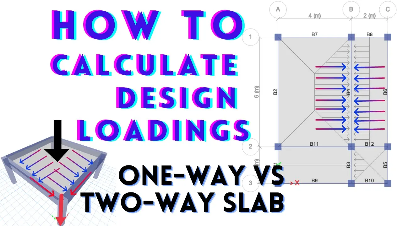
Basics of Structural Design Load Calculations | One-Way Vs Two-Way Slab
178.3K
Structures carry three basic types of loads: (1) Dead Load - the self-weight of the structure itself, (2) Superimposed Dead Load (SDL) - additional permanent loads like partitions, floor finishes, and MEP fixtures, and (3) Live Loads - movable or temporary loads such as furniture, people, and equipment. These loads are distributed through the structural system from slabs to beams, then to columns, and finally to footings resting on soil.
Click to watch →
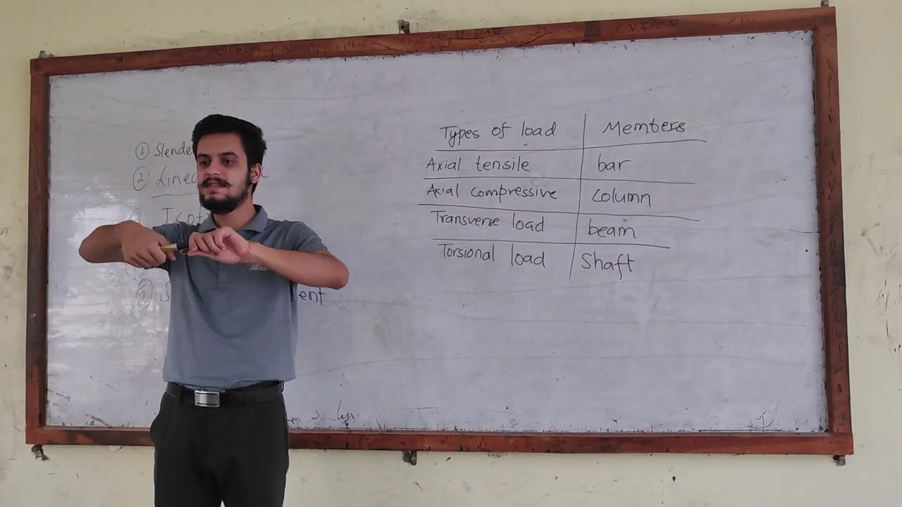
VID-2 | Types of support, FBD, Static indeterminacy of beams | CTEVT
212
Structural loads are classified based on their direction and application: (1) Axial loads act along the member's longitudinal axis - tensile loads pull members apart, compressive loads push them together; (2) Transverse loads act perpendicular to the axis, causing bending in beams; (3) Torsional loads cause twisting of members. The classification depends on the location of load application relative to the member's axis.
Click to watch →
SFD-BMD (PART-1 ) by Nikhil sir || GATE || SSC || STATE SSC || ESE
9.2K
There are five main types of loads in structural engineering: (1) Point Load - concentrated force at a single point, (2) Uniformly Distributed Load (UDL) - evenly distributed along the entire length, (3) Uniformly Varying Load (UVL) - changes uniformly along the length, (4) Non-uniform Distributed Load - varies irregularly, and (5) Couple - creates pure rotation without translation. Point loads are represented as arrows at specific locations. UDL is calculated as Total Load = w × L, where w is load intensity and L is length. UVL forms a triangular loading diagram.
Click to watch →

INTRODUCTION TO RC STRUCTURAL DESIGN (LOAD DECOMPOSITION TO BEAMS )
15.5K
Structures experience four main load types: Dead loads (permanent actions from self-weight of beams, slabs, finishes, fittings); Live loads (movable loads that can be dynamic or static like furniture and people); Wind loads (horizontal forces from wind on building surfaces, requiring zone-specific speeds); Seismic loads (earth crust vibrations during earthquakes). Codes specify different factors for each load type: BS uses 1.4 for dead and 1.6 for live, while Eurocode uses 1.35 and 1.5 respectively. Seismic design is typically required only for taller buildings.
Click to watch →
Deep Dive
Basic Mechanics of Materials: Concepts of tension, compression, shear force, and bending moments in structural elements.

Basic Mechanics of Materials Overview (Unit 7)
43K
This lecture covers the fundamental mechanical properties of materials, explaining that stress (force per unit area) and strain (deformation per unit length) are normalized measures that allow comparison across different specimen geometries, unlike raw force and deflection values. The course distinguishes between elastic behavior (reversible deformation where atoms stretch bonds and return to original positions) and plastic behavior (permanent deformation where atomic planes shear past each other). Key properties include Young's modulus (stiffness), Poisson's ratio (lateral contraction), yield stress (elastic-plastic transition), ultimate tensile strength, ductility (ability to stretch), toughness (energy to fracture), and hardness (resistance to indentation). The lecture also covers ceramic brittleness due to limited slip systems, polymer viscoelasticity with temperature-dependent behavior, and the use of safety factors in engineering design.
Click to watch →

BTSC JE 2025 Online Classes | BTSC JE Civil engineering Class | Mechanics of Material #Mrsstudy
157
This section covers the foundational concepts of Mechanics of Materials, including stress (force/area, units N/mm² or MPa), strain (change in length/original length, dimensionless), tensile and compressive stress, Hooke's Law valid up to elastic limit, Young's Modulus (stress/strain), Poisson's Ratio (lateral/longitudinal strain), relationships between elastic constants (E = 2G(1+ν), E = 3K(1-2ν)), thermal stress (σ = EαΔT), and compound bars where strain is uniform and load shares proportionally to Young's Modulus.
Click to watch →
Bienvenidos al mejor curso básico de mecánica de los materiales
8.5K
Mechanics of materials is the engineering discipline that studies how materials respond to applied forces, including stress and deformation under tension, compression, torsion, and flexion, as well as key mechanical properties like strength, stiffness, ductility, and hardness, and the theoretical foundations of elasticity and plasticity that explain reversible and permanent material deformation.
Click to watch →

ALL of AQA Materials in 24 Minutes | A Level Physics
1.1K
This comprehensive section covers the core mechanical properties essential for understanding material behavior. Beginning with density (mass/volume) and its application in ratio problems comparing different geometries, the content progresses to Hooke's Law establishing force-extension proportionality (F=kΔL) and identifying critical material limits—the limit of proportionality (where linearity breaks down) and the elastic limit (beyond which permanent deformation occurs). The section develops quantitative measures including tensile stress (force/area), tensile strain (extension ratio), and Young's modulus (stress/strain gradient). It explains how to determine Young's modulus graphically from force-extension curves. The treatment concludes with energy storage concepts (E=½FΔL=½k(ΔL)²) and distinguishes elastic recovery from plastic deformation, culminating in brittle material characteristics showing minimal plastic deformation before fracture.
Click to watch →

ليش بندرسها؟ | Mechanics of Materials
155
Mechanics of Materials is the science studying how solid objects behave under applied forces. The course explains why structures like bridges and buildings do not collapse. Key concepts include: (1) Types of deformation - compression, tension, bending, torsion, and fracture; (2) Stages of material failure - elastic deformation, yield point, plastic deformation, and fracture; (3) Stress (force per unit area) and strain (measure of deformation); (4) Material testing through stress-strain curves to determine mechanical properties; (5) Classification of materials as brittle (break suddenly) or ductile (deform before breaking); (6) Types of stresses - tensile, compressive, bending, torsional, and shear; (7) Buckling as a critical failure mode in slender columns under compression. Understanding these fundamentals is essential for preventing catastrophic failures in engineering designs.
Click to watch →
Deep Dive
Support Reactions: Familiarity with idealized structural supports (fixed, pinned, and roller joints) and how they constrain movement.

Resistência dos Materiais - Reações de Apoio - Aula 01
804K
To calculate support reactions in static structures, apply the equilibrium equations: sum of forces equals zero (ΣF = 0) and sum of moments equals zero (ΣM = 0). For a beam with supports A and B carrying a 10-ton point load at 6.5m from A and 2.1m from B, the reaction at B is calculated by taking moments about A: RB × 8.6m = 10t × 6.5m, yielding RB = 7.58 tons, and then RA = 10t - 7.58t = 2.42 tons.
Click to watch →
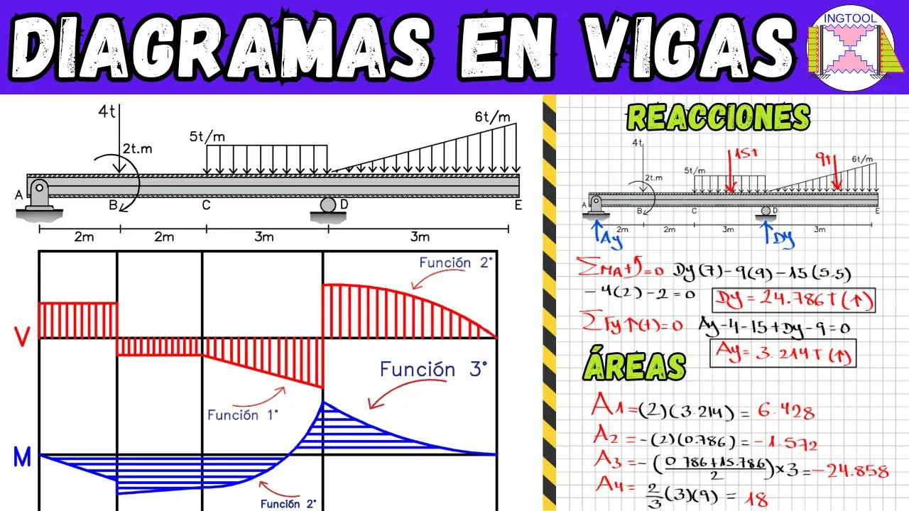
DIAGRAMAS DE FUERZA CORTANTE Y MOMENTO FLECTOR EN VIGAS FÁCIL Y RÁPIDO
100.6K
This segment covers the complete process of calculating support reactions for a beam. Fixed supports generate two reactions (vertical and horizontal), while roller supports generate only one vertical reaction. The horizontal reaction is determined by applying equilibrium conditions. The sum of moments about a point (counterclockwise positive equals zero) is used to solve for unknown reactions. Forces acting upward generate counterclockwise moments (positive), while forces acting downward generate clockwise moments (negative). For distributed loads, the resultant force equals the area (base × height for rectangular, base × height / 2 for triangular), with the center of gravity at the midpoint for rectangular loads and one-third from the right angle for triangular loads. Concentrated moments are added directly without multiplying by distance. The sum of vertical forces (upward positive equals zero) is then applied to find remaining reactions. Positive results confirm the assumed direction, while negative results indicate the opposite direction.
Click to watch →

HOW TO DRAW SFD AND BMD DIAGRAM SOLVED PROBLEM 6 IN HINDI | STRENGTH OF MATERIAL
134.6K
Support reactions are found using equilibrium conditions: ΣFy = 0 and ΣM = 0. For a simply supported beam, moment equation is applied at one support (e.g., point A). Clockwise moments are typically taken as positive. The moment equation includes all forces and their distances from the moment point.
Click to watch →

Engineering Mechanics: Statics Theory | Solving Support Reactions
70.9K
Three main support types exist in statics: (1) Pins restrict horizontal and vertical translation but allow rotation, providing two reaction forces (Ax, Ay); (2) Rollers restrict only one translation direction with reaction perpendicular to the surface; (3) Fixed connections restrict translation and rotation, providing three reactions (Rx, Ry, Mr). Simply supported beams combine pins and rollers for three total unknowns, solvable with three equilibrium equations.
Click to watch →

HOW TO DEAL MORE DAMAGE! (FROM 10K TO 200K) | Genshin Impact
720.3K
Support characters and elemental reactions are the most important and misunderstood aspects of maximizing damage in Genshin Impact. The video demonstrates that using the same character with identical weapons and artifacts can result in damage increasing from 10k to 200k (20 times more) simply by adding support characters. Bennett is considered broken because his ultimate provides massive damage buffs while healing. His artifacts should use a four-piece Noblesse set, and players should not invest heavily in his artifacts or level him beyond level 60. The Veredent set is essential for Electro characters as it increases swirl damage and decreases enemy elemental resistance.
Click to watch →
Prerequisite Knowledge
- Concept 01Fundamental Statics: Understanding static equilibrium, free-body diagrams, and force/moment balance.
- Concept 02Types of Structural Loads: Differentiating between dead loads (static weight of the structure) and live loads (moving traffic, wind, and environmental forces).
- Concept 03Basic Mechanics of Materials: Concepts of tension, compression, shear force, and bending moments in structural elements.
- Concept 04Support Reactions: Familiarity with idealized structural supports (fixed, pinned, and roller joints) and how they constrain movement.
Subsequent Learning
- Step 01AASHTO LRFD Bridge Design Specifications: Applying load distribution theories to official engineering codes and design methodologies.
- Step 02Finite Element Analysis (FEA): Using computational software (such as SAP2000 or ANSYS) to model and simulate complex bridge load paths.
- Step 03Seismic and Dynamic Analysis: Studying how bridge structures respond to dynamic, time-dependent forces like earthquakes, wind gusts, and aerodynamic flutter.
- Step 04Geotechnical and Foundation Engineering: Designing deep foundation systems (such as piles and caissons) and analyzing soil-structure interaction.
Load Transfer
Load Transfer
0:01Playing Section
- 1
Explains bridge load path from vehicles to ground.
- 2
Details roles of deck, beams, piers, and bearings.
- 3
Describes deep foundations for soft soil support.
Systemic Redundancy and Soil-Structure Interaction (SSI)
While classical structural engineering teaches a linear, sequential 'load path' where forces flow predictably from the deck down to the foundation, modern structural theory emphasizes Systemic Redundancy and Soil-Structure Interaction (SSI). This alternative perspective argues that treating bridge components as isolated, sequential transfer points oversimplifies reality. In actual practice, a bridge and the ground it rests upon form a highly coupled, non-linear feedback system. As foundations deform under load, soil-structure interaction dynamically redistributes stresses back up through the piers, bearings, and deck, altering the assumed load path. Furthermore, modern highly-redundant designs, such as integral (jointless) bridges, intentionally bypass traditional step-by-step load paths. Instead, they rely on monolithic behavior where the entire structure distributes loads globally. Relying solely on classical, static component-by-component load-path models can cause engineers to overlook these complex feedback loops, potentially leading to inaccurate safety margins or failing to predict progressive collapse paths under extreme dynamic forces.
Deep Dive
AASHTO LRFD Bridge Design Specifications: Applying load distribution theories to official engineering codes and design methodologies.
RD T1E12 - AASHTO LRFD Bridge Design Specifications
752
The AASHTO LRFD Bridge Design Specifications is a comprehensive 1900-page document that provides detailed guidelines for bridge design, covering multiple chapters including introduction and philosophy of design, load combinations and factors, structural analysis, reinforced concrete design, steel structure design, wood structure design, foundations, retaining walls, underground structures, railings, joints and bearings, and sound barriers; unlike general structural codes, this specification requires using both LRFD (Load and Resistance Factor Design) for strength limit states and ASD (Allowable Stress Design) for serviceability states such as fatigue, making it particularly important for bridges due to their critical role in regional connectivity and requiring significantly more verification effort than ordinary structures.
Click to watch →

Introduction and History of AASHTO LRFD Steel Bridge Design
5.2K
The AASHTO LRFD (Load and Resistance Factor Design) Bridge Design Specifications represent a comprehensive, probability-based design methodology that evolved from earlier Allowable Stress Design (ASD) and Load Factor Design (LFD) approaches. Developed through extensive research including the landmark AASHO Road Test (1956-1961) and NCHRP projects, LRFD was officially adopted in 1993 as the first calibrated reliability-based bridge design specification in the United States. The specification employs statistical calibration to achieve a target reliability index of 3.5, ensuring a more uniform level of safety across all bridge types and materials. It covers four primary limit states: Service (deflections, stress ranges), Fatigue (stress range limits), Strength (yielding, buckling, fracture), and Extreme Events (earthquakes, collisions). The LRFD approach was formally mandated for all new bridges starting October 1, 2007, replacing the traditional Standard Specifications.
Click to watch →

Lecture 2-1: Bridge Design Codes and Sources for Modular Bridge Design & Drawings
611
The ASHTO LRFD (Load and Resistance Factor Design) bridge design specification is published every 3-4 years with new versions. The 2007 fourth edition uses SI units, and all equations require compatible units—using FPS values with SI equations produces incorrect results. The code is organized into chapters covering introduction, joint design, loads, structure analysis, concrete and steel structures, and deck systems. While versions have minor differences (some sections removed or added), there are no significant changes between editions. The code serves as a comprehensive reference for bridge design but cannot be fully covered in a single lecture.
Click to watch →

AASHTO Committee on Bridges & Structures Overview
238
The AASHTO Committee on Bridges & Structures (COBBS) is a volunteer-based committee structure where state DOT personnel develop and update bridge design specifications through a formal ballot process; each state DOT can have up to three members on COBBS, with one designated as the voting member who participates in full committee voting on ballot items, while technical committees (such as T3 seismic design) meet regularly to develop proposals that are then voted on by the full committee before publication.
Click to watch →

DISEÑO DE PUENTE LOSA CON AASHTO LRFD 2014 - PLANTILLA EXEL 100% EDITABLE!!!
12.7K
This video presents an Excel template for designing simply supported bridge slabs following AASHTO LRFD 2014 standards, featuring automated calculations for dead load distribution factors, interior and edge strip moment analysis, HL-93 live load combinations with 33% impact factor, state limit verification (strength and service), fatigue assessment, and reinforcement distribution including main steel, distribution steel, and temperature reinforcement, with all parameters editable and color-coded for easy modification.
Click to watch →
Deep Dive
Finite Element Analysis (FEA): Using computational software (such as SAP2000 or ANSYS) to model and simulate complex bridge load paths.

Introduction to Finite Element Analysis | Basics
3.1K
Finite Element Analysis (FEA) is a numerical technique for finding approximate solutions to boundary value problems for partial differential equations. FEA and FEM (Finite Element Method) are the same concept, with FEA being the industry term and FEM being the academic term. FEA encompasses four main types of analysis: structural analysis (measuring structural behavior using linear and non-linear models), vibrational analysis (considering natural frequency and resonance to prevent structural failure), thermal analysis (predicting thermal stresses in steady and transient states), and fatigue analysis (predicting material life under cyclic loading). FEA is particularly valuable for solving complex problems with irregular geometry and complex boundary conditions, including solid mechanics, electromagnetic problems, and thermal analysis.
Click to watch →

Basics of CAE/FEA | CAE Interview Preparation | FEA Analyst | CAE Engineer | Stress Engineer Part -1
34.7K
Finite Element Analysis (FEA) is a numerical method that discretizes complex geometries into interconnected elements and nodes to solve partial differential equations. The method was pioneered in 1956 by Turner, Clough, Martin, and Topp, with the term 'finite element' coined by Ray Clough in 1960. FEA converts continuous mathematical models into solvable algebraic systems through stiffness matrices. The general equilibrium equation for dynamic analysis is M×acceleration + C×velocity + K×displacement = P(t), while static analysis simplifies to K×U = F. This foundational approach enables analysis across structural, thermal, fluid, and electromagnetic domains.
Click to watch →

FEA WEBINAR
1.1K
Finite Element Analysis (FEA) is a numerical method that transforms complex engineering problems into solvable matrix equations by discretizing continuous structures into finite elements, enabling engineers to analyze complex geometries, materials, and loading conditions that classical analytical methods cannot solve; the FEA process involves creating a mesh, applying boundary conditions and loads, solving equilibrium equations, and interpreting results, with accuracy depending on proper modeling techniques and validation against physical tests.
Click to watch →

Introduction to Finite Element Analysis (Part-1) | Skill-Lync
3.1K
Finite Element Analysis (FEA) is a numerical simulation technique that converts complex engineering problems into mathematical models by discretizing geometry into finite elements, applying partial differential equations and boundary conditions, and solving them to predict parameters like stress, displacement, and temperature; it enables engineers to validate designs virtually before physical prototyping, reducing development time and costs, with different analysis types including linear static analysis (valid below yield strength), nonlinear analysis (material/geometrical/contact), dynamic analysis (time-dependent), buckling analysis (compressive failure prediction), thermal analysis (temperature effects), and fatigue analysis (repeated loading).
Click to watch →

Session 02 : What is Finite Element Analysis | Ansys : Basic to Professional Course |
832
Finite Element Analysis (FEA) is a numerical method that solves engineering problems by discretizing continuous objects into smaller finite elements connected at nodes, reducing infinite degrees of freedom to finite values; this approach enables better visualization of failure locations, reduces design cycle time, decreases prototype numbers, and lowers testing costs through computational simulation.
Click to watch →
Deep Dive
Seismic and Dynamic Analysis: Studying how bridge structures respond to dynamic, time-dependent forces like earthquakes, wind gusts, and aerodynamic flutter.

🥾📐🏭Análisis Sísmico y Diseño de Edificios de Concreto Armado-Norma E030-E060-E020 / Etabs ✅🏙🌇
61K
This segment covers the assignment of seismic parameters, spectral analysis, and dynamic analysis methods. Seismic parameters include the seismic coefficient (Cs) calculated based on the structure's period and site conditions. For periods less than or equal to 0.5 seconds, Cs = 2.5; for periods between 0.5 and 2.5 seconds, Cs = 0.75 + 0.5 × T. The response spectrum defines the pseudo-acceleration for different periods of vibration, with the analysis involving defining the response spectrum function for each direction (X and Y) based on the site class and structural system. The software calculates the spectral acceleration for each mode of vibration, which is then used to determine the seismic forces on the structure. Dynamic analysis uses the response spectrum to calculate seismic forces for each mode of vibration, with modal combination methods (SRSS or CQC) to combine the effects of different modes. Torsional irregularity is verified by comparing the maximum displacement at one end of a floor to the average displacement at both ends. The maximum displacement must not exceed 1.3 times the average displacement. If this condition is violated, the structure is considered torsionally irregular.
Click to watch →

TALLER ACIPUCP:"Modelamiento y análisis sísmico de edificaciones de concreto armado con ETABS" (2/2)
5.3K
Dynamic analysis considers actual dynamic response to seismic ground motion, while static analysis uses equivalent static forces. The instructor demonstrates comparing dynamic and static base shear. Dynamic analysis should not produce base shear less than 80% of static analysis for regular structures. If it does, the dynamic analysis must be scaled up. The instructor shows how to create additional cases in ETABS to perform this comparison.
Click to watch →

IS 1893-2016( Seismic Load) Full Code Reading Video With Full Concept
228
Horizontal seismic coefficient (Ah) = (Z/2) × (I/R) × (Sa/G). Zone factor Z: 0.10 (Zone 2), 0.16 (Zone 3), 0.24 (Zone 4), 0.36 (Zone 5). Response reduction factor R: 3 for OMRF, 5 for SMRF. Importance factor I: 1 (<200 occupants), 1.2 (commercial), 1.5 (stadiums). Sa/G depends on time period (T=0.09H/√dx) and soil type. Dynamic analysis uses Response Spectrum Method (most common) and Time History Method. India's seismic zone map: Zone 2 (green, Z=0.10) includes Hyderabad, Aurangabad; Zone 3 (yellow, Z=0.16) includes Gujarat; Zone 4 (orange, Z=0.24) includes Srinagar; Zone 5 (red, Z=0.36) includes Shillong, Guwahati, Darbhanga. These zones determine seismic design parameters for structures across India.
Click to watch →

Asistente Sísmico E.030 2026 | Nuevas actualizaciones e interacción con ETABS
284
Dynamic seismic analysis requires modal analysis to achieve at least 90% mass participation in each direction according to code Article 40.2. The application shows how different numbers of modes affect mass participation. For this five-story building, 30 modes are required to achieve the 90% threshold in all directions. The seismic scaling factor is applied to dynamic analysis results to ensure the base shear meets minimum code requirements (80% for regular structures, 90% for irregular). The scaling factor is applied only to forces, not to displacements. Story drives (inter-story drifts) must be exported for derivation verification. The application creates two cases: one with un-scaled dynamic seismic loads and one with scaled dynamic seismic loads. Only the un-scaled case should be used for derivation analysis because the scaling factor applies only to forces, not to displacements.
Click to watch →

Complete Structural Analysis of Residential Building as per NBC 105:2020 (Equivalent Static Method)
59.8K
This section covers dynamic analysis setup for seismic evaluation. The video demonstrates configuring analysis options including output displacement types, torsion parameters, and center of mass calculation. Live load reduction factors are applied based on tributary area. Earthquake libraries provide predefined seismic parameters. The section explains how dynamic analysis evaluates structural response to lateral seismic forces and identifies potential torsional irregularities.
Click to watch →
Deep Dive
Geotechnical and Foundation Engineering: Designing deep foundation systems (such as piles and caissons) and analyzing soil-structure interaction.

MP Sub Engineer Vacancy 2026 | Paper Analysis (2016–2024) | notification big update 😱
127
Geotechnical Engineering includes Soil Mechanics and Foundation Engineering. Key chapters: Origin of soil and soil-water relationships, Classification of soil, Permeability, Compaction, Consolidation, Shear strength, Earth pressure and retaining walls, Slope stability, Deep foundations, Soil stabilization, Soil exploration. Six chapters are very important with many questions. Foundation Engineering also has many questions.
Click to watch →

GATE 2026 Syllabus | Civil Engineering | 150 Day Strategy To Score Single Digit Rank In GATE 2026
5.1K
Geotechnical Engineering (Soil Mechanics) and Foundation Engineering are essential branches of civil engineering. Soil Mechanics involves understanding soil behavior, soil testing, and determining if soil can support structural loads. Foundation Engineering is an advanced version of Soil Mechanics focusing specifically on foundation design. These subjects are industry-oriented and align with college curricula, with strong demand in the construction sector for soil testing and foundation work.
Click to watch →

What is Geotechnical Engineering?
269.9K
Geotechnical engineering is the branch of civil engineering that applies the mechanics of soils and rocks to the design and construction of foundations, earthworks, and other structures that interact with the ground, requiring site-specific investigations due to the highly variable nature of soil properties.
Click to watch →

Day 4 - Geotechnical Engineering | CTQ Demo | #bbmp #wrd #pwd #kea #kpsc #sscje #rrbje #ctq
151
Geotechnical engineering encompasses two main areas: Soil Mechanics and Foundation Engineering. Soil Mechanics deals with the properties of soil, while Foundation Engineering applies these properties to design foundations, determine bearing capacity values, calculate earth pressures behind retaining structures, and assess slope stability with factor of safety calculations.
Click to watch →
Foundation Engineering Course Introduction | What is foundation Engineering
2.4K
Geotechnical engineering, specifically foundation engineering, applies soil mechanics and rock mechanics principles to design foundation elements for structures. Foundations transfer structural loads to the ground, supporting diverse structures from bridges to skyscrapers. Key topics include soil exploration methods ranging from SPT to ground penetrating radar, slope stability analysis for hilly terrain modifications, earth pressure principles for retaining structures, bearing capacity determination for safe load application, and deep foundation solutions for weak strata. Real-world examples demonstrate these concepts in action across different structural applications.
Click to watch →
Load Transfer
Load Transfer
0:01- 1
Explains bridge load path from vehicles to ground.
- 2
Details roles of deck, beams, piers, and bearings.
- 3
Describes deep foundations for soft soil support.
Systemic Redundancy and Soil-Structure Interaction (SSI)
While classical structural engineering teaches a linear, sequential 'load path' where forces flow predictably from the deck down to the foundation, modern structural theory emphasizes Systemic Redundancy and Soil-Structure Interaction (SSI). This alternative perspective argues that treating bridge components as isolated, sequential transfer points oversimplifies reality. In actual practice, a bridge and the ground it rests upon form a highly coupled, non-linear feedback system. As foundations deform under load, soil-structure interaction dynamically redistributes stresses back up through the piers, bearings, and deck, altering the assumed load path. Furthermore, modern highly-redundant designs, such as integral (jointless) bridges, intentionally bypass traditional step-by-step load paths. Instead, they rely on monolithic behavior where the entire structure distributes loads globally. Relying solely on classical, static component-by-component load-path models can cause engineers to overlook these complex feedback loops, potentially leading to inaccurate safety margins or failing to predict progressive collapse paths under extreme dynamic forces.
Fundamental Statics: Understanding static equilibrium, free-body diagrams, and force/moment balance.
Types of Structural Loads: Differentiating between dead loads (static weight of the structure) and live loads (moving traffic, wind, and environmental forces).
Basic Mechanics of Materials: Concepts of tension, compression, shear force, and bending moments in structural elements.
Support Reactions: Familiarity with idealized structural supports (fixed, pinned, and roller joints) and how they constrain movement.
AASHTO LRFD Bridge Design Specifications: Applying load distribution theories to official engineering codes and design methodologies.
Finite Element Analysis (FEA): Using computational software (such as SAP2000 or ANSYS) to model and simulate complex bridge load paths.
Seismic and Dynamic Analysis: Studying how bridge structures respond to dynamic, time-dependent forces like earthquakes, wind gusts, and aerodynamic flutter.
Geotechnical and Foundation Engineering: Designing deep foundation systems (such as piles and caissons) and analyzing soil-structure interaction.
1.8K views21likes0:49@eazysurveysOriginal Release: 2026-05-28
A bridge is designed to safely transfer loads [music] from vehicles and people to the ground. Every part of the structure works together to move that weight downward into the soil. The deck is the surface where vehicles travel.
[music] It spreads the wheel loads from cars and trucks across a larger area so the structure below can safely carry them. Beams and girders support the deck, [music] transferring loads through bending moments and shear forces.
Piers and columns hold up the bridge span. They collect [music] the loads coming from the beams and transfer them further down into the foundation. Bridge bearings are placed between the beam and the pier. Their job [music] is to transfer loads while allowing the bridge to expand, contract, or slightly rotate due to temperature changes and traffic movement.
>> In areas with soft soil, [music] engineers use deep foundations such as piles. These piles transfer the bridge loads deep into strong soil or rock layers.
>> A safe bridge works because each component transfers loads step [music] by step from the deck to the beams to the piers and link the foundation and soil.
Up Next

24:09
Bridge Types and Engineering Design: A Structural Overview
@WIRED
966.2K views•2020-11-18

30:32
Ultrasonic Transducers: Resonant Frequency Measurement and Horn Design
@imajeenyus42
229.9K views•2017-02-22

54:16
Polymer Environmental Degradation: Mechanisms & Stabilization
@iit
1.8K views•2012-07-10

33:39
How a Student's Question Saved a NYC Skyscraper from Collapse
@veritasium
22.8M views•2025-04-26
Related Study Plans & Knowledge Roadmaps
Structured learning paths in Engineering
engineering
Building Acoustic Levitators: Physics & Arduino
01The Physics of Sound and Standing Waves
02Piezoelectric Transducers and H-Bridge Drivers
03Arduino Programming: Generating 40 kHz Signals
+ 2 more learning modules
14h5 modules
Explore Roadmap
engineering
Building Peltier Cloud Chambers: Particle Tracks
01Cosmic Rays & Cloud Chamber Physics
02Thermoelectric Cooling (TEC) Fundamentals
03Custom Liquid-Cooling Loop Design
+ 2 more learning modules
18h5 modules
Explore Roadmap
engineering
Yagi-Uda Antennas: Modeling, Build & VNA Test
01Introduction to RF and Antenna Fundamentals
02Yagi-Uda Antenna Design Principles
03Antenna Modeling and Simulation in 4NEC2
+ 2 more learning modules
18h5 modules
Explore Roadmap
engineering
ECG Monitor Design: Op-Amps, Filters & Noise
01Electronics & Breadboard Basics
02Op-Amps and Instrumentation Amplifiers
03Bioelectricity and ECG Fundamentals
+ 2 more learning modules
18h5 modules
Explore Roadmap