


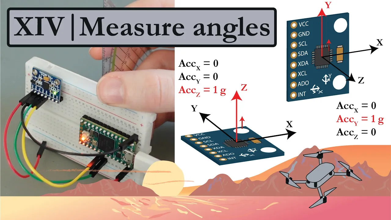
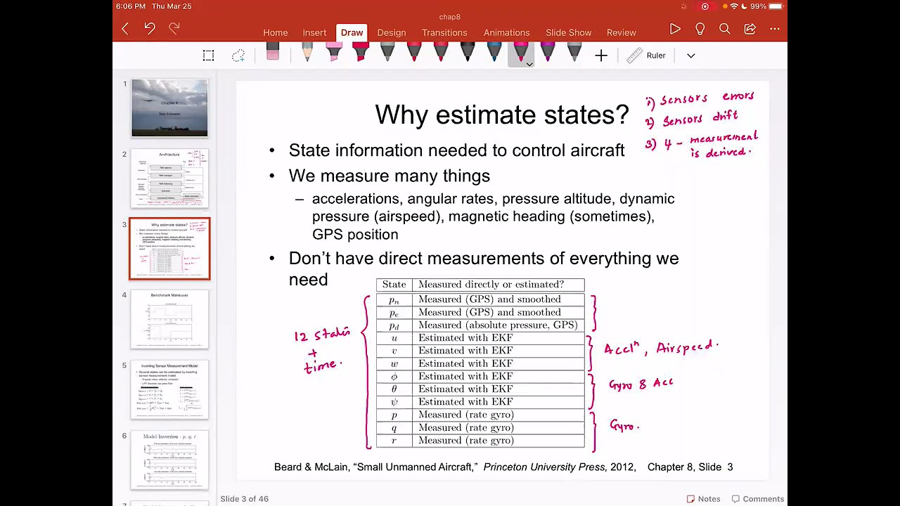
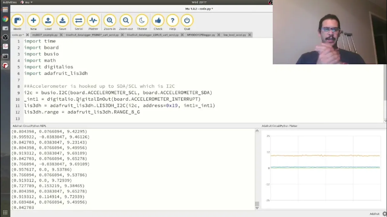
















A complementary filter combines accelerometer and gyroscope data by applying a low-pass filter to the accelerometer (which provides stable long-term orientation but has noise issues) and a high-pass filter to the gyroscope (which provides accurate short-term angular rate measurements but suffers from drift), using a weighted average formula θn = α×θ_prev + (1-α)×(θ_prev + ω×Δt) + (1-α)×θ_accel where α typically ranges from 0.96 to 0.98 to prioritize the gyroscope's short-term accuracy while allowing the accelerometer to correct for drift over time.
Complementary Filter for IMU Sensor Fusion | Lesson 11
Added:Fundamental understanding of how accelerometer and gyroscope sensors operate, including what physical quantities they measure (acceleration vs. angular velocity).
Familiarity with basic trigonometry and coordinate systems to calculate tilt (pitch and roll) from accelerometer gravitational vectors.
The concept of numerical integration (specifically, integrating angular velocity over time to estimate current angle).
Basic knowledge of signal noise, specifically distinguishing high-frequency noise (which affects accelerometers) from low-frequency bias/drift (which affects gyroscopes).
Introduction to mathematically optimal sensor fusion algorithms, such as the Kalman Filter and Extended Kalman Filter (EKF).
Exploring Madgwick and Mahony filters, which are highly efficient, industry-standard orientation algorithms.
Integrating a magnetometer (9-DOF sensor fusion) to correct for long-term heading (yaw) drift, which cannot be fixed by accelerometers alone.
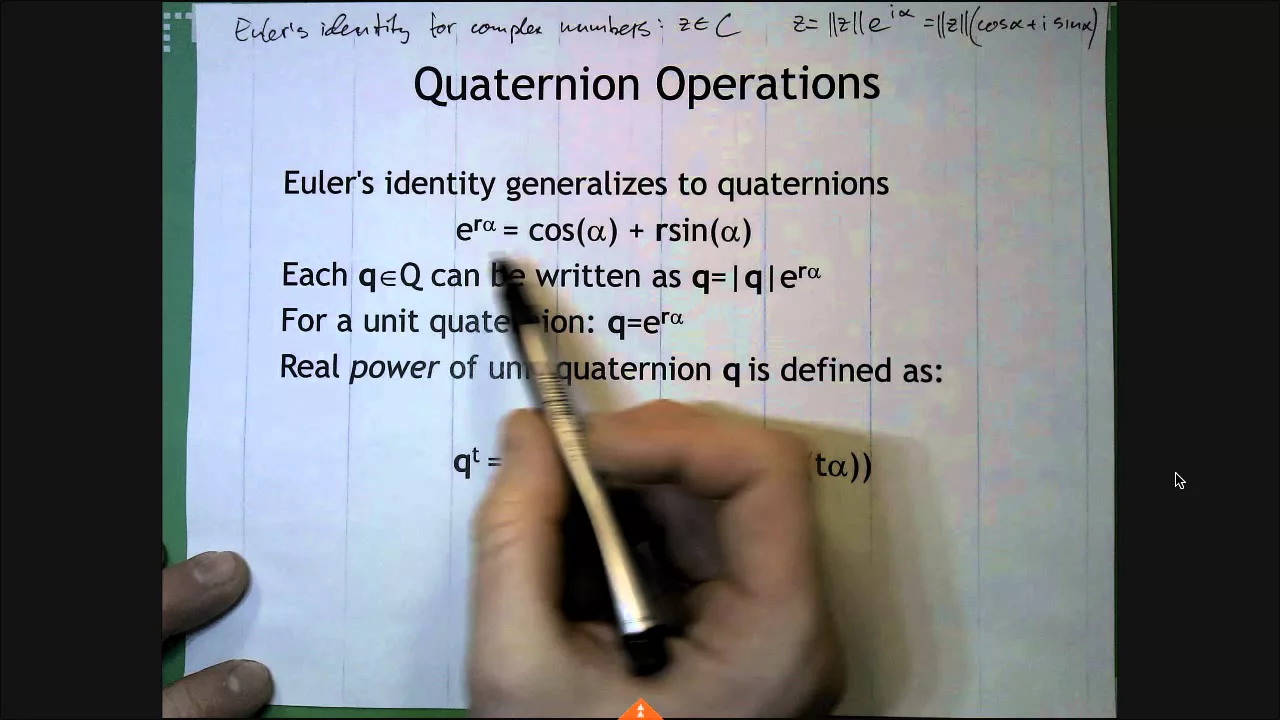
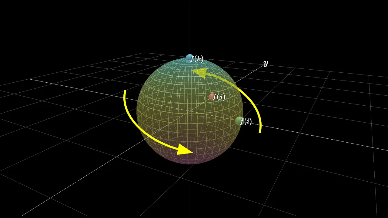
Studying Quaternions to represent 3D rotations, avoiding the mathematical limitation of gimbal lock inherent in Euler angles.
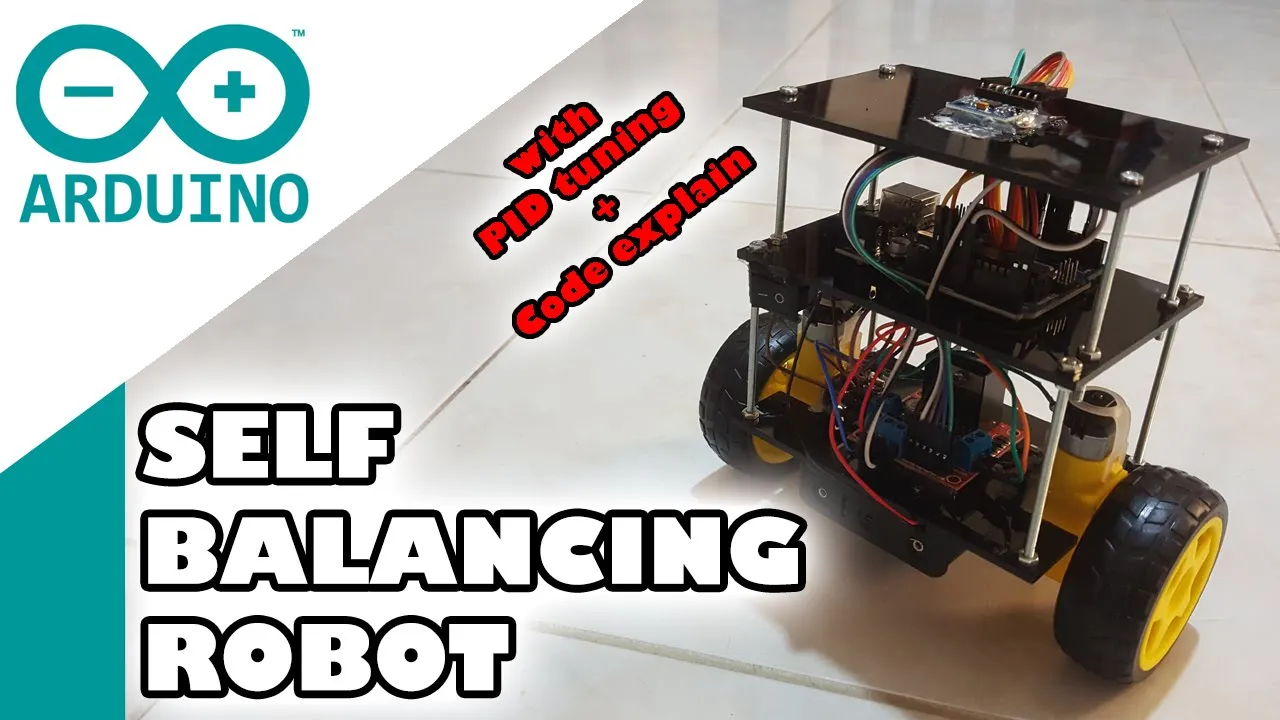
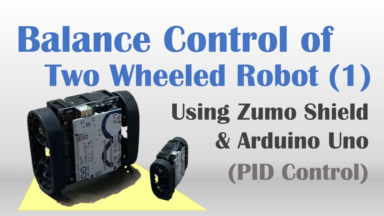
Applying estimated orientation to real-world control systems, such as PID controller tuning for self-balancing robots or quadcopter stabilization.
4.3K views86likes11:00Original Release: 2020-03-25
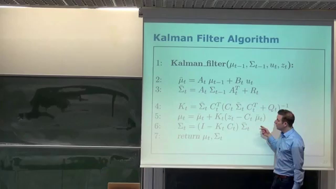
all right in this lesson then we're going to apply the complementary filter to our accelerometer and gyroscope data right we've seen that the accelerometer is a good indicator of angle orientation only when it's static right when it's not moving using the gravity vector so of course that doesn't help us on a moving robot we need something that's a good indicator dynamic conditions and that happens to be the gyroscope we just took a look at that in lesson 10 but we also saw with a gyroscope then that we have a problem of drift right over time there's this DC offset our air that gets integrated into our measurement and it then what drift means is if we start with one position we move around and we come back to the same position that drift error will say we're not it will not give us the same position right it will be off so we want to be able to try and get rid of some of that drift air and we want to take the but the best of both the best of the accelerometer which over the longer term gives us a more stable gives us a stable acceleration vector in terms of where we are angle wise that's really allows the explanation of that alright the accelerometer over the long term will give us a good measurement of our angle if we can filter out the effects of any vibration and we've seen with accelerometer that if we use something like a low-pass filter on it then we can get rid of some of that fine noise with the gyroscope right the gyroscope works best in the dynamic condition right it's calm it's constantly changing it's a higher frequency change so the gyroscope needs basically a high-pass filter with it so what a complementary filter does is it takes the best of both worlds and put a complementary filter uses two filters that complement each other so if you think about it then a low-pass filter and a high-pass filter are complements of each other because we know the low-pass filter then only allow signals that are less than this corner frequency basically to pass in a high-pass filter doesn't pass signals that are lower than its corner frequency only higher right and so what this signal flow diagram is saying is if we feed then the accelerometer angle and through a low-pass filter and we feed the gyro right if we integrate that over the sample time so that we can get the angle from the gyro run that through a high-pass filter some of these two together in effect we're passing both frequencies both signals but we're cleaning them up right and so it complements each other so we're going to see that this alpha this weighting factor that we use here which is very familiar from the low-pass filter that we take a look at is going to weight how much we say in how much we trust one signal over another over the short term right so here's the general form then right we say that the overall the output of the filter theta n is equal to this alpha the scaling factor times theta so the angle the filtered angle output that we had at the time before the sample before we're going to add to that the gyro rate so the state of gyro is the gyro rate we just read times the sample time interval so there's that integration step right we get degrees per second times seconds this gives us degrees so units of degrees here we're going to add to that right one minus alpha and so these values alpha plus 1 minus alpha have to sum to 1 right so alpha is always going to be something less than or equal to 1 and greater than or equal to zero all right so 1 minus alpha times the reading that we get from the accelerometer in the sample interval so that's our general form of our complimentary filter right and we want to take a look at them if we look at this equation we say well how is that a low-pass and how is that a high-pass filter how is that doing it so what we want to do is if we look at this formula and we're going to assume the gyroscope reading is zero right we're in it so if the gyroscope reading is zero that means we're in a steady state right we've only got the accelerometer data coming in from the formula because if we zero this out right what we have here is we have sometimes the angle the filter to angle output from the time before the sample before so notice the gyro data zero that's why that term is missing plus one minus alpha times the accelerometer data right and if you look at this form this is the very same form that we've used for a low-pass filter that we previously studied right the formant that form that we looked at is we said well the output Y was multiplied by the current input X so X for the input value so think that this is the accelerometer input times 1 minus alpha there's that term and then what we added to that before was the previous filtered output there's the previous filtered output times alpha that's how this acts as a low-pass filter is if we think of the gyro as being 0 if we take out the effective gyro from that we can see that that is low-pass filtering than this portion of the accelerometer angle this walks through as well if you wanted to convert then this equation to its Z transform right this is what this is doing it's taking this equation so here's the same thing down here and if we want to put it the Z domain I we know that the N minus 1 becomes the Z minus 1 term we pull that out so we actually then have this in the form of theta right its sample Z is alpha times Z minus 1 times theta z plus 1 minus alpha times this and from the accelerometer right at times Z and then I'm pulling out then both of these theta terms so we're moving this to the other side of the equation here so we have both of the filtered output terms on this side but we have the accelerometer on this side and so we want to put this in the form of a transfer function then the output right over the input that relationship here becomes 1 minus alpha over 1 minus alpha right the scale or 1 minus alpha times right that time delay right we have that's the previous sample like that so that's the minus 1 that's your time delay I and if you then also want to relate this to the time constant that we talked about before with a low pass filter right the time constant knew that should be tau this shows us T approximate approximately equals this formula it's not exactly it's close enough so if you want to calculate alpha based on what you want your time constant to be right here's your formula that you use alpha times delta T divided by 1 minus alpha where delta T is your sampling period and then if we want to think about how does the time constant tau relate to noise the easiest way is to think of an example as an example so suppose our sampling frequency was 100 Hertz a hundred times a second we read this that means our sampling period is 10 milliseconds if we set alpha equal to a 0.8 our time constant is 40 milliseconds right plugging things in to this formula what that means is that any noise that is shorter in duration than 40 milliseconds will be removed so that's how we can think about the time constant in terms of how we're sampling this and how often we're sampling this in practice what you're going to find is that alpha a lot of times is 0.9 or higher because the gyroscope will be giving us good information actually for this particular filter you might find that 0.96 to 0.98 works fairly well for alpha because the gyroscope will give us the best measurement in the short term the other thing is then how does it act as a high-pass filter well we start with that original equation right and we're going to remove the accelerometer signal from that right assume that the accelerometer signal is zero at that point we're going to leave only the effect of the gyroscope signal so our formula reduces to this right our filtered output is equal to alpha times the previous filtered output plus the gyro rate the current driver rate times the sample time and if you look at the general form of a high-pass filter well that's amusing eyes here and my VY is equal to alpha times so why is the output so the filtered output is equal to alpha times the previous filtered output alpha times the previous filter output plus alpha times the change in input values well here's alpha times the change in input values that theta dot that's our change for the previous time so this then does act as a high-pass filter like I just said before alpha values are usually large because we want the gyro to have a short term effect on the angle estimation the smaller weight on the accelerometer actually then has a longer term effect of getting rid of the drift right there getting rid of some of that any of that noise that might be in there from the DC offset if you look at the lesson ten video after I moved my unit around my mpu sixty fifty and we let it sit for a while we can see that at first the drift was large and then the drift was getting smaller and smaller as it just sat there statically of course your robot can't just sit there forever and hope the drift will come back but what you're going to see in your homework assignment hopefully is you're going to implement now the complimentary filter right you're going to compare that against what you're getting out of accelerometer what you're getting out of the gyroscope and see which gives you the best results hopefully the complimentary filter will do that there are some other filters that are more complex to implement remember we're running this on an Arduino microcontroller so we want something quick and dirty not a whole lot of math right we need that our code to fly across that microcontroller we implement something say like a common filter it's a little more complex to understand I probably will talk about it later in the course but for right now this filter should do really well for our IMU all right so I will see everybody in the next unit I believe this is the end of our unit on the IMU right we're going to start moving on to motors control systems obstacle detection after this
Up Next
9:41
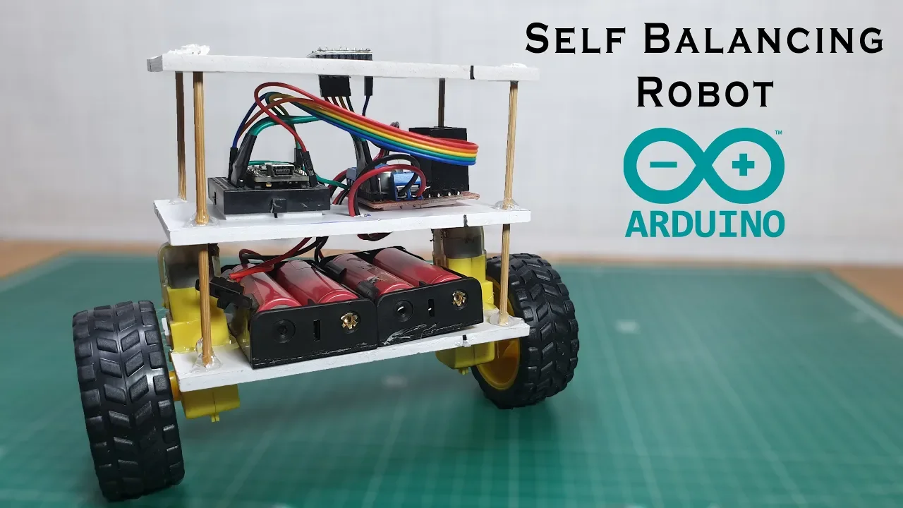
Arduino Self-Balancing Robot: DIY Build with MPU6050
@ViralScience
91.7K views•2019-12-01

58:25
MathWorks Virtual RoboSub Simulation Environment | Webinar 2026
@RoboNationInc
209 views•2026-03-10

11:04
How to Build a Self-Balancing Robot: Arduino Nano & MPU6050
@easytechzones
16.8K views•2022-03-09

25:22
Micromouse: The Fastest Maze-Solving Robots on Earth
@veritasium
23.5M views•2023-05-24
Related Study Plans & Knowledge Roadmaps
Structured learning paths in Robotics
robotics
Building Delta Robots: Kinematics & Pico
01Foundations of Delta Robots & Mechanical Design
02Electronics and Microcontroller Setup with Pi Pico
03Delta Robot Kinematics and Coordinate Math
+ 3 more learning modules
65h6 modules
Explore Roadmap
robotics
Building Ballbots: Dynamics, Kalman & LQR
01Embedded Electronics & Omniwheel Actuation
02Ballbot Kinematics & Rigid Body Dynamics
03IMU Sensors & Kalman Filter State Estimation
+ 2 more learning modules
42h5 modules
Explore Roadmap
robotics
Micromouse: Hardware, PID Control & Flood-Fill
01Electronics & Teensy Microcontroller Basics
02Sensors and Actuators: Motors, Encoders & IR
03Precision Movement: Implementing PID Control
+ 2 more learning modules
35h5 modules
Explore Roadmap
robotics
CDPR: Kinematics, Arduino & Winch Control
01Foundations of Arduino & Basic Electronics
02Stepper Motors and Winch Mechanics
03Kinematics of 2D Cable-Driven Robots
+ 2 more learning modules
28h5 modules
Explore Roadmap