A self-balancing robot uses an Arduino microcontroller to read sensor data from an MPU-6050 accelerometer/gyroscope, then adjusts motor speeds through an L298N motor driver to maintain balance by counteracting any detected tilt or fall.
Arduino Self-Balancing Robot: DIY Build with MPU6050
Added:Deep Dive
Basic Arduino programming and familiarity with the IDE, including GPIO configuration, PWM signals, and the I2C communication protocol.

Arduino DE #2 IDE, Pinbelegung
542
This tutorial covers the complete Arduino setup process: downloading and installing the Arduino IDE software from the official website, connecting the Arduino board via USB to the PC, uploading a test sketch to verify the connection, customizing IDE preferences such as line numbers and sketch storage location, and understanding the Arduino board's pin configuration including power pins (5V, 3.3V, GND), digital pins (0-13) with special functions like PWM and interrupts, analog pins (A0-A5) for reading sensor values, and communication interfaces like I2C.
Click to watch →

2- التعرف على الأردوينو | Introduction to Arduino
3.3K
Arduino programming uses a C/C++-based language called Arduino language, with programs called 'sketches' written in the Arduino IDE. The IDE interface includes a title bar, menu bar, toolbar, and code editing area with default code. The Setup section runs once at startup for configuration (like setting pin modes), while the Loop section runs continuously in a repeating cycle for main program logic. Pin configuration uses pinMode(pinNumber, MODE) where MODE is INPUT or OUTPUT. Pins 0-1 are reserved for serial communication.
Click to watch →

Home Automation, Smart City | Application of IoT Part 1 | iot
182
The Arduino IDE provides a beginner-friendly programming environment supporting C/C++ syntax with automatic indentation, brace matching, and syntax highlighting features. The built-in LED on Arduino Uno is controlled by pin 13, where high voltage (1) turns it off and low voltage (0) turns it on. Power can be supplied through USB or external 7-12V sources, with the onboard regulator generating 3.3V. Pins can be configured as input or output using pinMode(), with digitalWrite() controlling voltage levels and delay() managing timing intervals. A complete blinking program initializes pin 12 as output in setup(), then alternates between HIGH and LOW states in loop() with 5000ms delays. This foundational programming pattern enables extension with environmental sensors to create responsive smart lighting systems.
Click to watch →
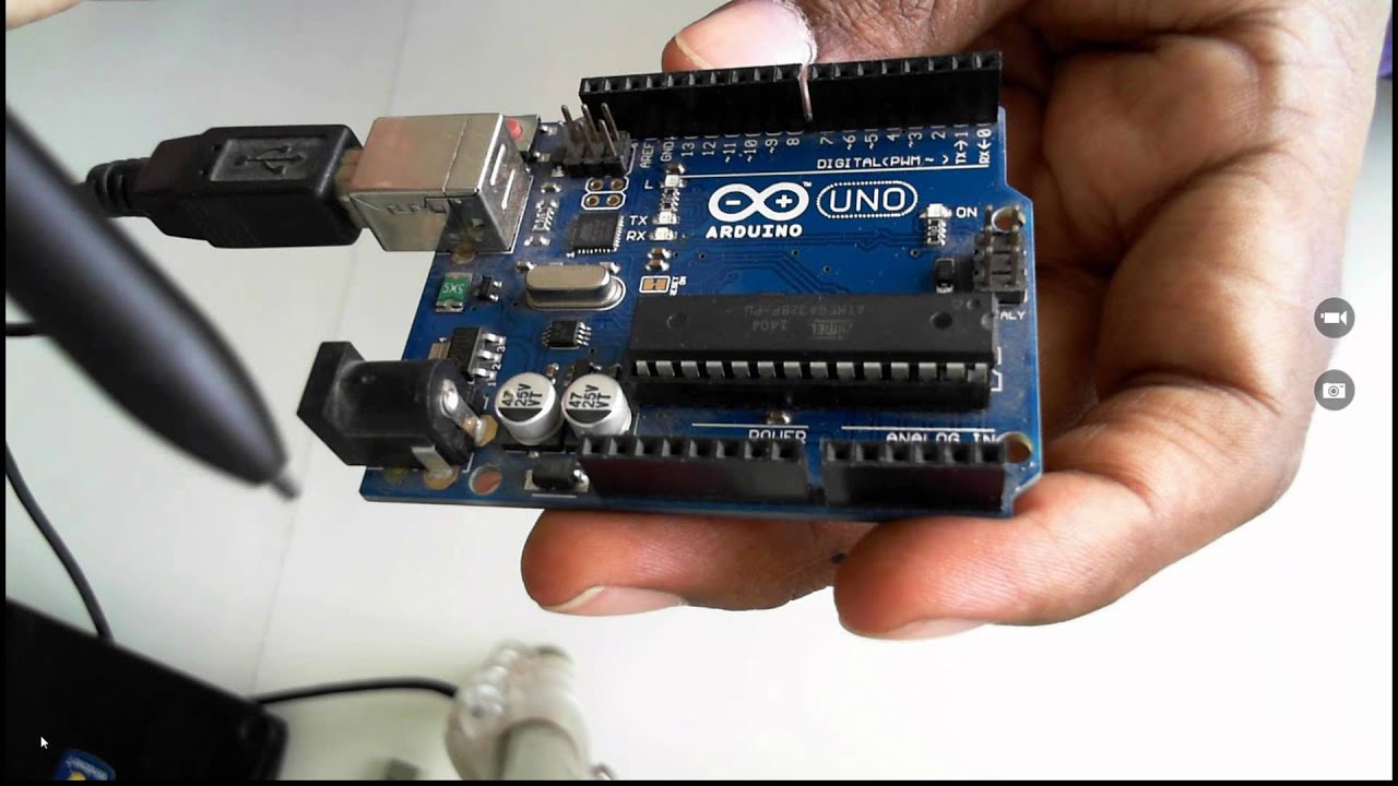
Beginning with Internet of Things IoT for Developers
171.5K
Arduino programming uses C-based sketches written in a simplified version of C. The Arduino IDE provides tools for writing, compiling, and uploading code to the board. The IDE includes a Serial Monitor for viewing output. Arduino programs have only two main constructs: setup() (runs once at startup) and loop() (runs continuously). Built-in functions include pinMode() for configuring pins as input or output, digitalWrite() for writing values to digital pins, and delay() for introducing time delays in milliseconds. Libraries are pre-written code that simplifies working with sensors and components, handling complex communication protocols and data interpretation.
Click to watch →

3. The Arduino IDE
42.9K
Arduino provides comprehensive I/O functions: pinMode() sets pin direction (INPUT, OUTPUT, INPUT_PULLUP); digitalWrite() sets pin state; digitalRead() reads pin state; pulseIn() measures pulse duration; tone() generates square waves; noTone() stops tones. Analog functions include analogReference() for setting reference voltage and analogRead() for 10-bit ADC readings (0-1023). The analogWrite() function generates PWM signals (500 Hz, 8-bit resolution) for simulating analog output. Advanced features include interrupts for event-driven processing, bit manipulation functions, and TWI/I2C interface for multi-device communication.
Click to watch →
Deep Dive
Fundamental principles of DC motors and how H-Bridge motor drivers (like the L298N) regulate motor direction and speed.

DC Motor Drivers: H-Bridge Control with Arduino Guide
853.9K
DC motors operate on simple principles: applying voltage causes rotation in one direction, reversing polarity reverses rotation. Selecting appropriate motor drivers requires matching three key specifications: motor voltage, average current under normal load, and stall current during shaft seizure. H-bridge configurations are the standard solution for bidirectional motor control, using four switches arranged in an H-shape. The L298N represents a foundational dual H-bridge motor driver capable of handling motor voltages from 5 to 35V with continuous current up to 2A and peak current up to 3.5A. It accepts logic voltage from 3.3 to 5V and can derive logic power from the motor supply when voltage exceeds 7.5V. The driver employs bipolar transistor technology, resulting in inherent inefficiency with approximately 1.4V total voltage drop across the bridge, necessitating large heatsinks and making it unsuitable for battery-powered applications.
Click to watch →
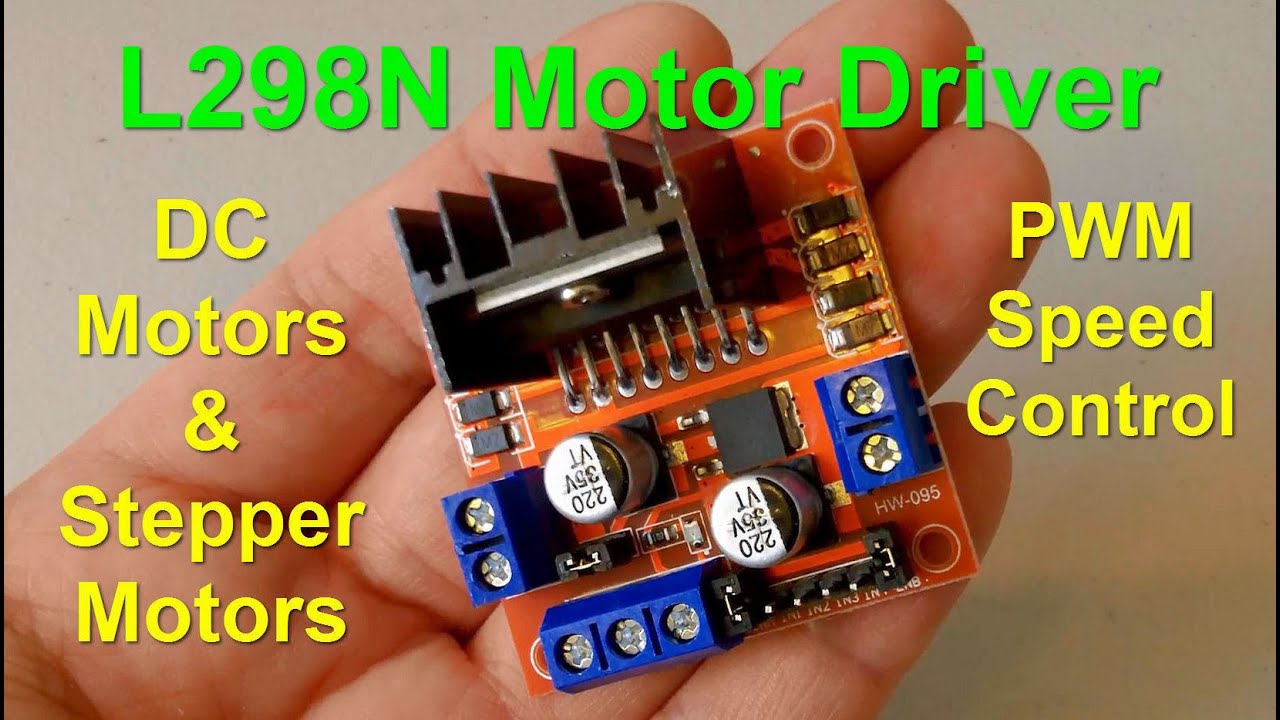
L298N Dual H-Bridge Motor Driver for DC and Stepper Motors
207.2K
The L298n dual H-bridge motor driver is a versatile module that controls two DC motors (up to 2A each) or one stepper motor using TTL signals; it features a 5V regulator with a jumper for power supply management (7-12V with jumper enabled, >12V requires external 5V), where direction is controlled by IN1-IN4 inputs (high for forward, low for reverse) and speed via PWM when enable jumpers are removed, while stepper motors require specific pulse sequences (e.g., 1-3-2-4 for clockwise, reversed for counterclockwise) applied to the phase connectors.
Click to watch →
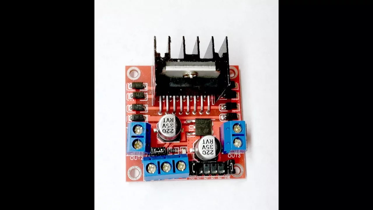
The L298N H-bridge motor controller module - basics
92.1K
The L298N is a dual full-bridge motor controller module that can drive one servo or two DC motors, accepting input voltages from 5-35V DC with a recommended 7-12V range; it features an internal 5V regulator that requires a minimum 7V input to function properly, and controls motor direction through input pins (IN1-IN4) while speed is regulated by the input voltage, with enable pins (A and B) controlling whether each motor set responds to input signals.
Click to watch →
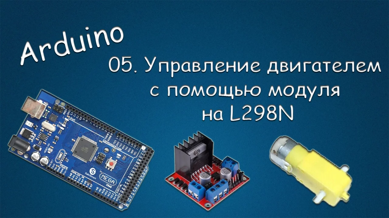
#071 ARDUINO 05 Управление двигателем с помощью модуля на L298N
45K
The L298N H-bridge module enables control of DC motor direction and speed through two control inputs (IN1 and IN2) for direction and PWM signals on enable pins for speed regulation. When IN1 and IN2 have opposite states, the motor rotates in one direction; when both are high or both low, the motor stops. Speed is controlled by varying the PWM duty cycle on the enable pins, which adjusts the average voltage delivered to the motor. The module includes a built-in 5V regulator for logic power and protective diodes for motor back-EMF protection.
Click to watch →

✅ El más usado en Robótica para controlar Motores DC, Motores de Pasos, Driver L298N Puente H
264.8K
The L298N is a dual H-bridge motor driver that controls DC motors by managing direction through two input pins (IN1/IN2 for motor A, IN3/IN4 for motor B) and speed through PWM signals on enable pins (ENA/ENB), with voltage control ranging from 5-35V depending on jumper settings.
Click to watch →
Deep Dive
The physics of Inertial Measurement Units (IMUs), specifically how accelerometers and gyroscopes measure tilt angle and angular velocity.

Intro to Inertial Measurement Units (IMU)
46.1K
An Inertial Measurement Unit (IMU) is a sensor system that measures orientation and motion using gyroscopes (which detect angular rotation rates but suffer from bias and drift requiring correction algorithms like Kalman filters) and accelerometers (which measure linear acceleration including gravity to determine tilt angles but require filtering to reduce noise); IMUs are classified by their sensor accuracy, with hobbyist-grade units having biases around 0.01g and 100°/hour, while high-end aerospace IMUs achieve biases below 0.00001g and 0.1°/day, and sensor fusion techniques combine multiple sensor readings to improve overall measurement accuracy.
Click to watch →

9-Axis IMU LESSON 6: Determine Tilt From 3-axis Accelerometer
36.2K
Proper IMU calibration requires systematic procedures: gyroscope self-calibrates when stationary, magnetometer calibrates through multi-directional motion, and accelerometers require 45-degree and upside-down orientations. Real-world applications include drop detection for laptop hard drive protection, airbag deployment systems that distinguish crashes from curb hits, and vehicle hill steepness measurement. The geometric foundation relies on the constant downward gravity vector intersecting sensor axes at varying angles, creating a right triangle where the hypotenuse represents gravity (1g) and the adjacent/opp sides represent axis-specific accelerations.
Click to watch →

CHARLA EN VIVO, Acerca de sensores INerciales (IMU) y su uso en navegación
846
Unmanned vehicle navigation requires establishing a Cartesian coordinate system and calculating orientation angles. The Inertial Measurement Unit (IMU) consists of accelerometers and gyroscopes. Accelerometers measure acceleration and detect gravity to calculate roll and pitch angles but cannot measure yaw. They are sensitive to vibrations and rapid movements. Gyroscopes measure angular velocity in all three axes, providing 6 degrees of freedom when combined with accelerometers. However, gyroscopes suffer from drift, where small measurement errors accumulate over time, causing calculated angles to drift away from true values.
Click to watch →

How a Quadcopter Works - Flight Mechanics, Components, & Sensors (2)
95.5K
The IMU (Inertial Measurement Unit) contains two sensors: the accelerometer measures linear force exerted on the quad (linear acceleration), and the gyroscope measures rotational motion. Together, they measure linear and rotational forces but do not know the absolute position or orientation (whether the quad is upright or upside down).
Click to watch →

Inertial Measurement Unit (IMU) – A tiny sensor system with wide range of applications
693
An Inertial Measurement Unit (IMU) detects and measures movement in three-dimensional space using accelerometers, gyroscopes, and optionally magnetometers. Accelerometers measure linear acceleration along three axes (X, Y, Z), providing three degrees of freedom. Gyroscopes measure angular rotation around three axes (roll, pitch, yaw), adding three more degrees of freedom. Combined, these create six-axis IMUs; adding a magnetometer creates nine-axis IMUs for Earth magnetic field orientation. MEMS (Micro-Electro-Mechanical Systems) combines mechanical and electronic components in microscopic packages. MEMS accelerometers use suspended proof masses with polysilicon springs; acceleration causes displacement changing capacitance between electrodes. MEMS gyroscopes use the Coriolis effect: oscillating proof masses experience perpendicular forces during rotation. Structures are 100 times smaller than human hair (hundreds of nanometers to 300 micrometers), enabling fast response and mass production. Tuning fork configurations ensure angular rotation detection independent of linear acceleration.
Click to watch →
Deep Dive
An introductory understanding of feedback control loops, specifically the conceptual framework of a PID (Proportional-Integral-Derivative) controller.

PID Loop Basics - NO MATH!
8.1K
A PID (Proportional-Integral-Derivative) control loop is a feedback mechanism that adjusts an output to maintain a control variable at a desired setpoint; the Proportional component multiplies the error (difference between actual and desired values) by a gain factor to produce an immediate corrective output, the Integral component accumulates past errors over time (measured in seconds) to gradually increase output until the setpoint is reached, and the Derivative component predicts future errors based on the rate of change to minimize response time and eliminate dead time, with all three components working together to achieve precise and stable control in industrial and HVAC applications.
Click to watch →

Le PID: Introduction
28.4K
This comprehensive section covers the foundational concepts of feedback control systems. It explains the basic structure including the process (plant), sensor, reference input, comparator, and controller generating control action u. The feedback loop enables continuous comparison between actual and desired performance. The section introduces PID control combining proportional (current error), integral (accumulated past errors), and derivative (rate of error change) terms. The mathematical formulation u(t) = Kp×e(t) + Ki×∫e(t)dt + Kd×de(t)/dt is presented, explaining how each term addresses different aspects of system behavior. The section establishes why pure proportional control has limitations in eliminating steady-state error and preventing oscillations, motivating the need for the complete PID approach.
Click to watch →

PID For Robot Control Part 1
24.5K
A PID (Proportional-Integral-Derivative) feedback loop is a control system that continuously monitors a system's state through sensors, calculates the error between the current state and the desired goal, and uses a mathematical function to adjust actuators, creating an infinite loop that maintains the system at the target state despite external disturbances.
Click to watch →

What is a PID Controller?
29K
A PID (Proportional-Integral-Derivative) controller is a feedback mechanism that maintains a system at its desired setpoint by combining three control actions: Proportional control applies corrective force proportional to the current error (how far off-target the system is), Derivative control applies force based on the rate of change of error (how fast the system is moving away from target), and Integral control applies force based on the accumulated error over time (to eliminate steady-state offset). Together, these three components work to reject disturbances and bring the system back to the target position, with each component addressing different aspects of system behavior—proportional handles immediate error, derivative prevents overshoot by anticipating future error, and integral eliminates long-term drift.
Click to watch →

PID control explained clearly (Beginner's Guide)
970
A feedback loop continuously measures output using sensors, compares it to a set point, and makes corrections through a repeating cycle of measure, compare, and correct. PID control combines three actions: Proportional reacts to current error distance, Integral addresses accumulated error over time, and Derivative responds to rate of change. Together they reduce deviation from the set point. Proportional alone causes oscillation with overshoot and undershoot. Integral gradually eliminates steady-state error by tracking accumulated offset. Derivative anticipates overshoot by reacting to approaching changes. Modern controllers can auto-tune to optimize these parameters automatically.
Click to watch →
Prerequisite Knowledge
- Concept 01Basic Arduino programming and familiarity with the IDE, including GPIO configuration, PWM signals, and the I2C communication protocol.
- Concept 02Fundamental principles of DC motors and how H-Bridge motor drivers (like the L298N) regulate motor direction and speed.
- Concept 03The physics of Inertial Measurement Units (IMUs), specifically how accelerometers and gyroscopes measure tilt angle and angular velocity.
- Concept 04An introductory understanding of feedback control loops, specifically the conceptual framework of a PID (Proportional-Integral-Derivative) controller.
Subsequent Learning
- Step 01Advanced PID tuning methodologies, including mathematical modeling of the robot's physics and implementing auto-tuning algorithms.
- Step 02Implementing sensor fusion techniques, such as Kalman filters or Complementary filters, to merge accelerometer and gyroscope data for cleaner readings.
- Step 03Integrating wireless communication modules (like HC-05 Bluetooth or ESP32 Wi-Fi) to enable remote steering and telemetry monitoring.
- Step 04Upgrading to optical encoder-equipped DC motors or stepper motors to achieve precise position control and dead reckoning (odometry).
- Step 05Exploring more complex dynamic stability projects, such as reaction wheel pendulums, ballbots, or bipedal walking platforms.
Creative Hub
Visual Feats
Core Concepts
Practical Twists
Final Showcase
Creative Hub
0:01Playing Section
- 1
Channel presents science-driven creative content.
- 2
Focuses on innovation and visual engagement.
- 3
Sets tone for upcoming visual demonstrations.
Limitations of Classical PID and 8-bit Hardware in Modern Robotics
While the Arduino, MPU6050, and L298N combination is a popular introductory DIY project, experienced roboticists often criticize it as an outdated and inefficient paradigm for learning modern control systems. The L298N motor driver is highly inefficient, wasting significant power as heat and causing voltage drops. The 8-bit Arduino microcontroller lacks the processing speed and hardware floating-point unit required for high-frequency sensor fusion and advanced control loops. Furthermore, basic Proportional-Integral-Derivative (PID) controllers struggle with non-linear dynamics under external disturbances. Modern robotics engineering favors 32-bit microcontrollers (such as ESP32 or STM32) paired with high-efficiency motor drivers, and utilizes Linear Quadratic Regulator (LQR) state-space control instead of PID. LQR provides a mathematically optimal control strategy that analyzes the entire state of the system simultaneously, offering far superior stability, robustness, and educational value for modern control theory.
Deep Dive
Advanced PID tuning methodologies, including mathematical modeling of the robot's physics and implementing auto-tuning algorithms.
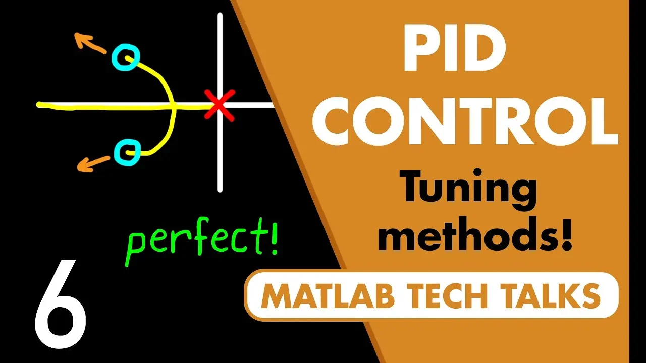
Manual and Automatic PID Tuning Methods | Understanding PID Control, Part 6
291.1K
With a mathematical model of a physical system, PID controllers can be tuned systematically rather than through trial-and-error. The process involves replacing the physical plant with its mathematical description, then using control theory methods to derive appropriate controller gains. The goal is to obtain gains that work for the physical system when the model is sufficiently accurate. This approach contrasts with brute-force manual tweaking and leverages control theory principles for more reliable results.
Click to watch →
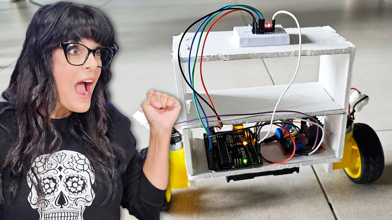
Build a Self-Balancing Robot with Arduino for Beginners
61.1K
Successful PID tuning requires patience and systematic adjustment. Start with KP=0 and KI=0, then incrementally increase KP from 10 to 25, watching for the first successful self-correction. Once KP is approximately correct, adjust KD (starting around 1.2) to dampen overcorrections. Only change one parameter at a time, making small incremental changes rather than large jumps. Initial falls are expected and indicate progress. The key indicator is whether the robot catches itself at least once when released. After KP and KD are approximately correct, adjust KI (starting around 0-80) to eliminate long-term drift.
Click to watch →
A PID Tuning Guide | Understanding PID Control, Part 4
349.9K
Manual tuning techniques for model-based PID include pole placement (placing closed-loop poles at desired locations), loop shaping using Bode/Nyquist plots to shape frequency response, and heuristic methods applied to simulation. Automatic tuning algorithms implement established heuristics within software, generating initial gain sets that typically require manual refinement. Auto-tuning can operate on models, combine with system identification using input-output data, or run in real-time on hardware. Despite automation capabilities, manual tweaking remains essential for achieving precise desired responses. This flexibility makes PID particularly valuable for well-behaved systems where users can later adjust gains for specific situations without requiring extensive control theory knowledge.
Click to watch →
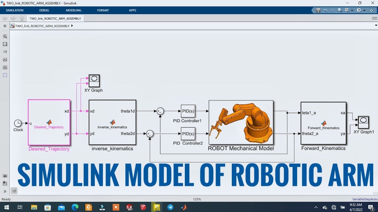
The Full Modeling and simulation of a Robotic Arm using MATLAB simscape multibody and Solidworks
164.8K
This extensive section covers the complete development of a robot control system, from block configuration through advanced PID tuning. Students learn to configure Simscape Multibody blocks including clock blocks for time-based trajectory generation, XY Graphs for visualization, PID Controller blocks for each joint, and Sum blocks for error computation. The section covers configuring revolute joints for actuation and sensing, using PS-Simulink converters, and creating subsystems to organize complex models. Students implement inverse kinematics as MATLAB Function blocks, writing custom code to convert desired Cartesian coordinates (xd, yd) to joint angles (theta1, theta2) using geometric relationships with defined link lengths. Forward kinematics computes Cartesian positions from joint angles for visualization. The section addresses debugging challenges including undefined variables, syntax errors, and connectivity verification. Students then master PID controller tuning: manual tuning starting with proportional gain to reduce steady-state error, introducing integral gain to eliminate remaining error while monitoring overshoot and settling time. The section demonstrates automated tuning using MATLAB's PID Tuner app, which linearizes the nonlinear mechanical model and provides slider-based adjustment of response characteristics. Critical computational trade-offs are addressed: derivative action provides stability but consumes significant CPU resources, requiring students to balance tracking accuracy against computational efficiency by setting D=0 or using PI control when necessary.
Click to watch →
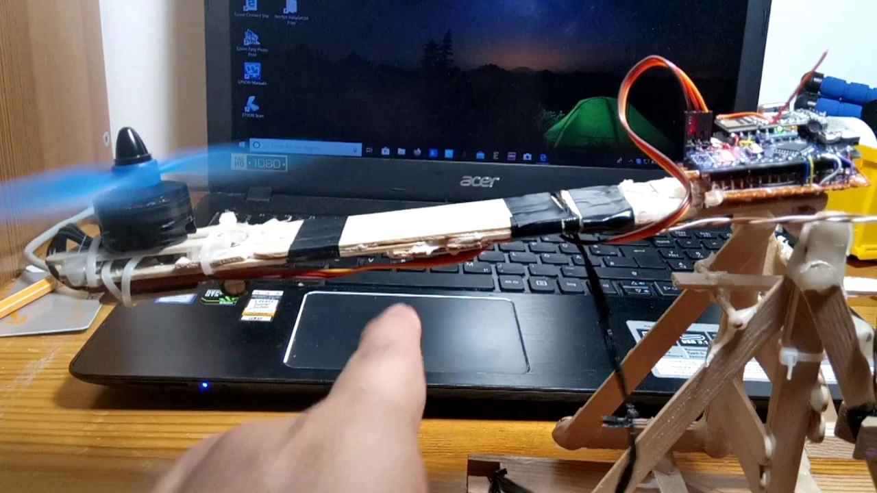
WAJIB Tonton! Penjelasan PID
19.2K
Three modeling approaches exist for PID tuning: Black box (no internal knowledge, only input-output observation), Grey box (partial knowledge of parameters like motor rotation per degree), and White box (complete mathematical model including all physical parameters like voltage effects, temperature influences, and mechanical properties). Each approach balances complexity against accuracy. Black box is simplest but least precise, while white box requires detailed physical understanding. The choice depends on available resources and required control precision.
Click to watch →
Deep Dive
Implementing sensor fusion techniques, such as Kalman filters or Complementary filters, to merge accelerometer and gyroscope data for cleaner readings.
(Sponsored) Complementary Filter - Sensor Fusion #2 - Phil's Lab #34
56.4K
The complementary filter is a computationally efficient sensor fusion technique that combines accelerometer and gyroscope data to estimate roll and pitch angles by exploiting their complementary strengths: accelerometers provide stable long-term estimates when the system is at rest (measuring gravity), while gyroscopes offer accurate short-term angular rate measurements without drift; the filter merges these estimates using a weighted combination where the weighting factor alpha (typically 0.02-0.05) determines how much trust is placed in each sensor, with lower values favoring gyroscope estimates and higher values favoring accelerometer estimates.
Click to watch →
(Sponsored) Accelerometers and Gyroscopes - Sensor Fusion #1 - Phil's Lab #33
123.4K
Sensor fusion combines accelerometer and gyroscope data to improve attitude estimation accuracy, as accelerometers drift during dynamic motion while gyroscopes suffer from long-term drift; this complementary approach addresses the limitations of using either sensor alone for reliable orientation tracking in applications like UAVs.
Click to watch →
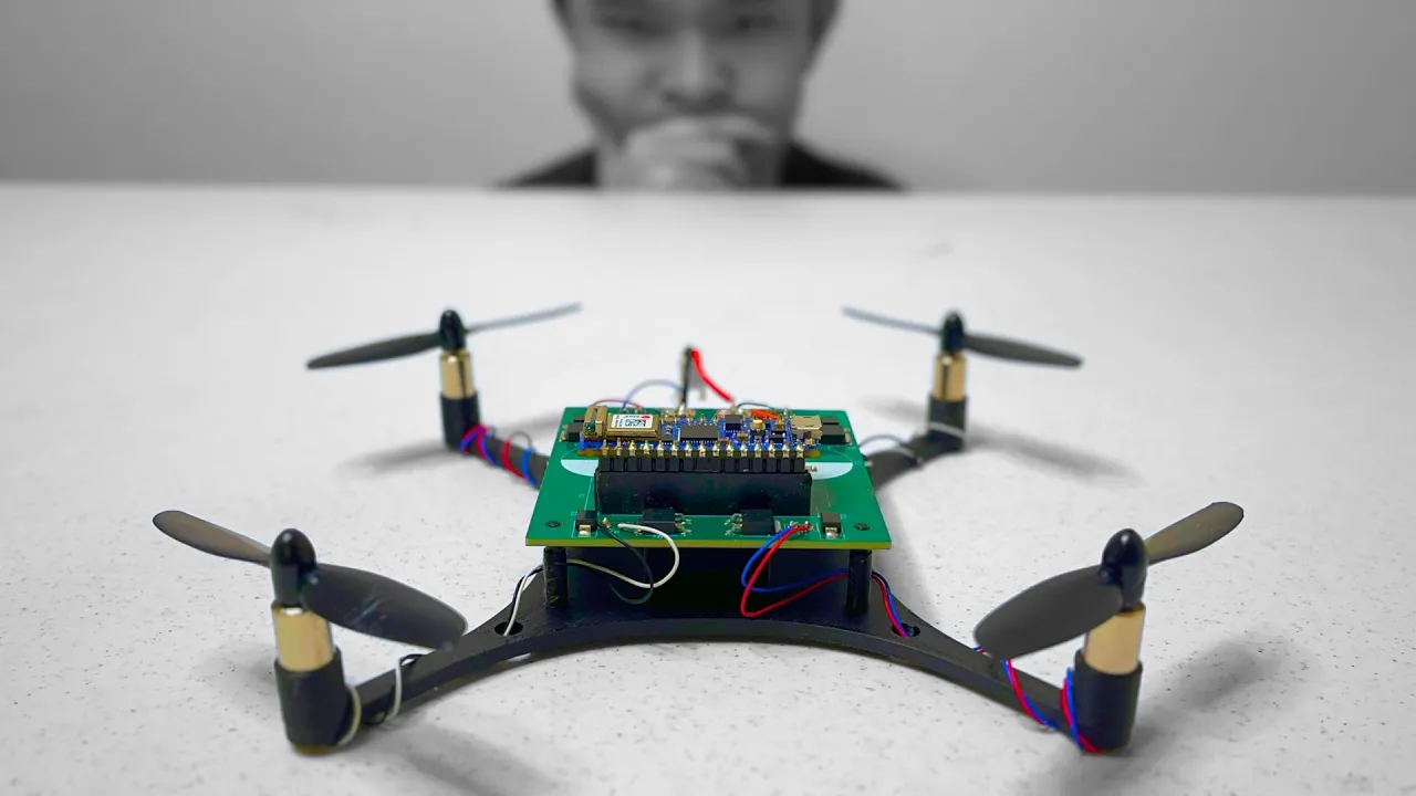
I Attempted to Design my Own Drone... with SUPERCAPACITORS
138.9K
A complementary filter combines gyroscope and accelerometer data to improve angle measurement accuracy. The process involves taking raw gyroscope values, multiplying by time between readings to get degrees traversed, then adding this to the final angle calculation. For the accelerometer portion, trigonometry calculates tilt angles based on acceleration measurements. The final angle combines mostly gyroscope data (for short-term responsiveness) with a small portion of accelerometer data (for long-term stability), creating sensor fusion.
Click to watch →
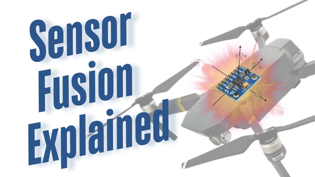
How sensor fusion works? - Simple explanation
20.9K
Sensor fusion combines data from multiple sensors (gyroscope and accelerometer) to achieve more accurate and reliable measurements than either sensor could provide alone; the complementary filter achieves this by taking a weighted average of the gyroscope's smooth but drifting angle measurements and the accelerometer's noisy but stable angle measurements, with an optimal gain value around 0.91-0.96 that balances noise reduction and drift minimization for stable drone flight.
Click to watch →

Speedrunning My Engineering School Project on the Last Day
81.8K
This segment demonstrates how to combine multiple sensors to overcome individual limitations through sensor fusion. The complementary filter algorithm recursively combines gyroscope and accelerometer data: it calculates angle changes from gyroscope angular velocity, adds to previous estimates, then combines with accelerometer data using weighted averaging (90% gyroscope, 10% accelerometer). This approach leverages the gyroscope's short-term accuracy while using the accelerometer to correct long-term drift. The filter acts as a low-pass filter, allowing stable low-frequency signals while attenuating high-frequency noise. The result is a filtered angle that closely matches the encoder's direct measurement while being applicable to applications where encoders cannot be used, such as drones. This technique is fundamental in robotics, navigation, and autonomous systems.
Click to watch →
Deep Dive
Integrating wireless communication modules (like HC-05 Bluetooth or ESP32 Wi-Fi) to enable remote steering and telemetry monitoring.
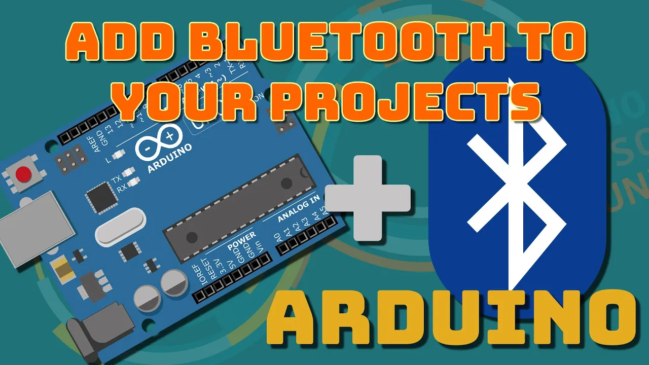
Adding Bluetooth to Your Arduino Project with an HC-05 or HC-06 Bluetooth Module
142.6K
This tutorial demonstrates how to add wireless Bluetooth connectivity to Arduino projects using HC-05 or HC-06 modules, covering hardware wiring with voltage level conversion (using a 2.2kΩ and 5.7kΩ resistor divider for 3.3V to 5V conversion), software setup using the SoftwareSerial library to create a serial communication channel on pins 8 and 9, and establishing connections through a mobile phone Bluetooth terminal app for bidirectional data transmission between the Arduino and mobile device.
Click to watch →

APM Flight Controller DIY HC 12 Serial Telemetry Module for Mission Planner Waypoint Mission
12.5K
Implement HC05 Bluetooth module as relay between HC12 and devices. Connect HC05 to FTDI, enter AT command mode by holding button during USB connection. Set HC05 baud rate to 38400 (default), then change to 57600 using AT+UART=57600,0,0. Connect HC05 RX to HC12 TX and vice versa. Power both modules via ST-Link. On computer, select Bluetooth COM port at 57600 baud in Mission Planner. For mobile access, pair HC05 via Bluetooth settings (default password '1234'), install Mission Planner on phone, select paired module, set baud rate to 57600, and connect. Execute arm/disarm commands from mobile device for complete wireless control capability.
Click to watch →

Lesson #6: Internet of Things (IoT): ESP8266 and Bluetooth module HC05
198
The HC-05 Bluetooth module enables wireless communication between microcontrollers and smartphones, operating at 5V with 30mA current consumption and 9600 baud rate using UART protocol; it connects via four wires (5V to VIN, GND to GND, TX to GPIO 5 as RX, RX to GPIO 4 as TX) and can be controlled through Arduino IDE using SoftwareSerial library to transmit and receive data, enabling applications like remote LED control systems.
Click to watch →
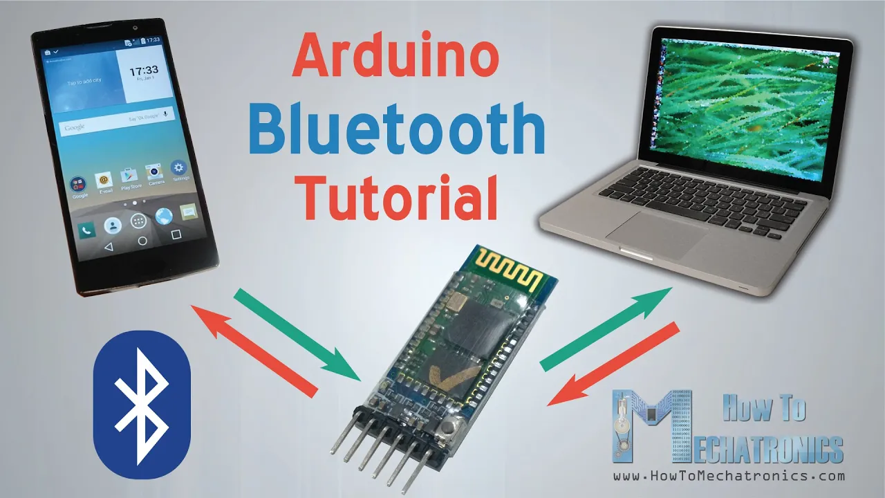
Arduino and HC-05 Bluetooth Module Tutorial | Android Smartphone & Laptop Control
729.1K
The HC-05 Bluetooth module enables wireless serial communication between Arduino boards and external devices such as smartphones or laptops by transmitting data through serial communication at a default baud rate of 38,400; when connecting to devices with different voltage levels (like 5V Arduino to 3.3V Bluetooth module), a voltage divider is required on the TX line to prevent damage, and the communication protocol involves sending ASCII characters (e.g., '0' for off, '1' for on) which are read by the Arduino and used to control connected components like LEDs.
Click to watch →

HC-05 vs HC-06 vs HM-10 vs ESP32 | Which Bluetooth Module Should You Use?
195
The best Bluetooth module depends on your specific project requirements rather than a universal 'best' choice; HC-05 offers maximum flexibility as a master/slave module with customizable settings, HC-06 is simpler and cheaper for basic phone-controlled applications, HM-10 provides low-power Bluetooth 4.0 but may be complex for beginners, RN-42 is industrial-grade but expensive and overkill for simple projects, while ESP32 integrates Wi-Fi and Bluetooth in a single microcontroller at lower cost than separate modules.
Click to watch →
Deep Dive
Upgrading to optical encoder-equipped DC motors or stepper motors to achieve precise position control and dead reckoning (odometry).
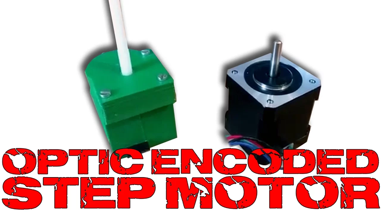
Build an optic encoded HIGH precision step motor
78.3K
An optic encoder converts angular motion into digital pulses by using an infrared LED and photo transistor to detect holes and fields on a rotating disc, enabling precise control of motor rotation angle, speed, and position through step counting; the system requires proper resistor values to ensure voltage levels meet microcontroller logic thresholds and the optic switch must operate at frequencies compatible with motor speed.
Click to watch →

✅ Encoder para sentido de giro de motor dc
15.2K
This comprehensive project demonstrates precise DC motor control using optical encoders for exact positioning. The system uses a H-bridge circuit with relays for bidirectional motor control, dual optical encoders (A and B) for position and direction detection, and limit switches for safety boundaries. Single sensors cannot determine rotation direction; two sensors with a specially designed disk (larger slot spacing) enable direction detection by comparing which sensor triggers first. The ESP32 microcontroller manages all connections with internal pull-up resistors. The program uses step-based counting (44 steps = 11 revolutions) instead of time-based control for reliable positioning regardless of load variations. This architecture enables precise control for applications like stage lighting systems where accurate positioning is critical.
Click to watch →
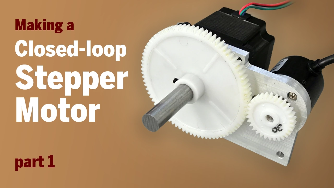
Converting a Stepper Motor to a Closed-loop Stepper Motor - Part 1
345.7K
A closed-loop stepper motor can be created by attaching an optical rotary encoder to a standard stepper motor's shaft, enabling position feedback for precise control; this mechanical modification involves extending the motor shaft, designing a custom mounting plate with CNC machining, and preparing mounting holes and threads to secure both the motor and encoder together.
Click to watch →

How to use encoders (Optical, Hall Effect, Quadrature)
135K
Encoders are electromechanical devices measuring angular position through rotating discs and sensors. Single-phase encoders provide basic rotation detection but cannot determine direction. Optical encoders use infrared LEDs and receivers separated by slotted discs, producing square wave outputs where high states indicate light passing through slots and low states indicate blocking. This fundamental principle enables pulse counting for RPM calculation and position tracking.
Click to watch →

Control Large DC Motors with Arduino! SyRen Motor Driver Tutorial
516.7K
DC gear motors can achieve positional accuracy similar to stepper or servo motors by adding an encoder. An encoder provides feedback about the motor's actual position, enabling closed-loop control that ensures precise positioning. This transforms a simple DC motor into a synthetic device capable of accurate location control, expanding the capabilities beyond basic speed control to include precise positioning applications.
Click to watch →
Deep Dive
Exploring more complex dynamic stability projects, such as reaction wheel pendulums, ballbots, or bipedal walking platforms.
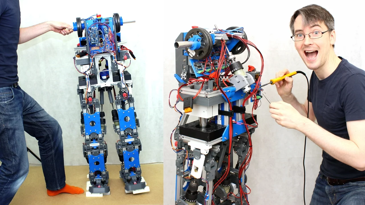
Building Robot X #6 | More Dynamic Stability | James Bruton
79.4K
This video demonstrates how dynamic stability in bipedal robots can be achieved through multi-axis control systems that integrate inertial measurement units (IMUs) with feedback-driven actuators. The presenter builds upon previous work by adding front-to-back stability using a dedicated actuator controlled by an IMU, addressing issues of rocking and oscillation caused by loose actuators. Key innovations include differential gain control between hip and ankle joints to prevent tipping, leg bending mechanisms that absorb impact loads, and hard end stops on rubber feet to maintain consistent ground contact. The robot demonstrates the ability to stabilize itself dynamically in motion by measuring its orientation in space and coordinating all eight motors to dampen unwanted movement, showing that effective bipedal stability requires simultaneous control across multiple axes with carefully tuned feedback loops.
Click to watch →

Péter Fankhauser: Meet Rezero, the dancing ballbot
132.8K
Ballbots are robots that balance and move on a single ball, achieving dynamic movement through inherent instability; they maintain balance by continuously measuring their pitch angle and counteracting toppling via motor adjustments at 160 times per second, while three wheels on the ball enable omnidirectional movement and rotation.
Click to watch →

Could Alien Tripods really walk Robot
362.5K
Reaction wheels spin a large mass around a stationary center point to create reaction forces that push the robot in the opposite direction. By measuring the robot's angle and dynamically controlling the reaction wheel speed, a device can actively balance itself. This principle is used in balancing robots and can be applied to tripod robots to allow them to balance on two legs while taking steps with the third leg.
Click to watch →

Android 12 Part 7, Initial Dynamic Stability Testing for my bipedal humanoid android
17.2K
This video demonstrates how a bipedal humanoid robot achieves dynamic stability through the integration of multiple RC gyroscopes (Hobby King HK 401) wired in series with servo motors, where gyroscopes on the thighs, knees, and ankles continuously monitor angular motion and compensate for disturbances by adjusting servo positions to maintain balance during movement.
Click to watch →

HAL9000 : Ball Balancing Robot
194.7K
Ball-balancing robots require dynamic stability to remain upright, which means they must continuously adjust their motor speeds and positions approximately 100 times per second. This rapid adjustment is necessary because any imbalance causes the robot to tip over. The system reads data from an inertial measurement unit (IMU) containing both a gyroscope and accelerometer, then uses a controller to make real-time adjustments to all six axes of motion simultaneously.
Click to watch →
Creative Hub
Visual Feats
Core Concepts
Practical Twists
Final Showcase
Creative Hub
0:01- 1
Channel presents science-driven creative content.
- 2
Focuses on innovation and visual engagement.
- 3
Sets tone for upcoming visual demonstrations.
Limitations of Classical PID and 8-bit Hardware in Modern Robotics
While the Arduino, MPU6050, and L298N combination is a popular introductory DIY project, experienced roboticists often criticize it as an outdated and inefficient paradigm for learning modern control systems. The L298N motor driver is highly inefficient, wasting significant power as heat and causing voltage drops. The 8-bit Arduino microcontroller lacks the processing speed and hardware floating-point unit required for high-frequency sensor fusion and advanced control loops. Furthermore, basic Proportional-Integral-Derivative (PID) controllers struggle with non-linear dynamics under external disturbances. Modern robotics engineering favors 32-bit microcontrollers (such as ESP32 or STM32) paired with high-efficiency motor drivers, and utilizes Linear Quadratic Regulator (LQR) state-space control instead of PID. LQR provides a mathematically optimal control strategy that analyzes the entire state of the system simultaneously, offering far superior stability, robustness, and educational value for modern control theory.
Basic Arduino programming and familiarity with the IDE, including GPIO configuration, PWM signals, and the I2C communication protocol.
Fundamental principles of DC motors and how H-Bridge motor drivers (like the L298N) regulate motor direction and speed.
The physics of Inertial Measurement Units (IMUs), specifically how accelerometers and gyroscopes measure tilt angle and angular velocity.
An introductory understanding of feedback control loops, specifically the conceptual framework of a PID (Proportional-Integral-Derivative) controller.
Advanced PID tuning methodologies, including mathematical modeling of the robot's physics and implementing auto-tuning algorithms.
Implementing sensor fusion techniques, such as Kalman filters or Complementary filters, to merge accelerometer and gyroscope data for cleaner readings.
Integrating wireless communication modules (like HC-05 Bluetooth or ESP32 Wi-Fi) to enable remote steering and telemetry monitoring.
Upgrading to optical encoder-equipped DC motors or stepper motors to achieve precise position control and dead reckoning (odometry).
Exploring more complex dynamic stability projects, such as reaction wheel pendulums, ballbots, or bipedal walking platforms.
91.7K views1.3Klikes9:41@ViralScienceOriginal Release: 2019-12-01
[Music] viral science be home of creativity [Music] [Music] [Music] [Music] [Music] [Music] [Music] [Music] [Music] [Music] [Music] do subscribe and press Bell icon to get instant notification for new video [Music]
Up Next

8:18
How to Create and Set Up a ROS2 Workspace | ROS2 Tutorial
@RoboticsBackEnd
134K views•2022-08-17

58:25
MathWorks Virtual RoboSub Simulation Environment | Webinar 2026
@RoboNationInc
209 views•2026-03-10

11:04
How to Build a Self-Balancing Robot: Arduino Nano & MPU6050
@easytechzones
16.8K views•2022-03-09
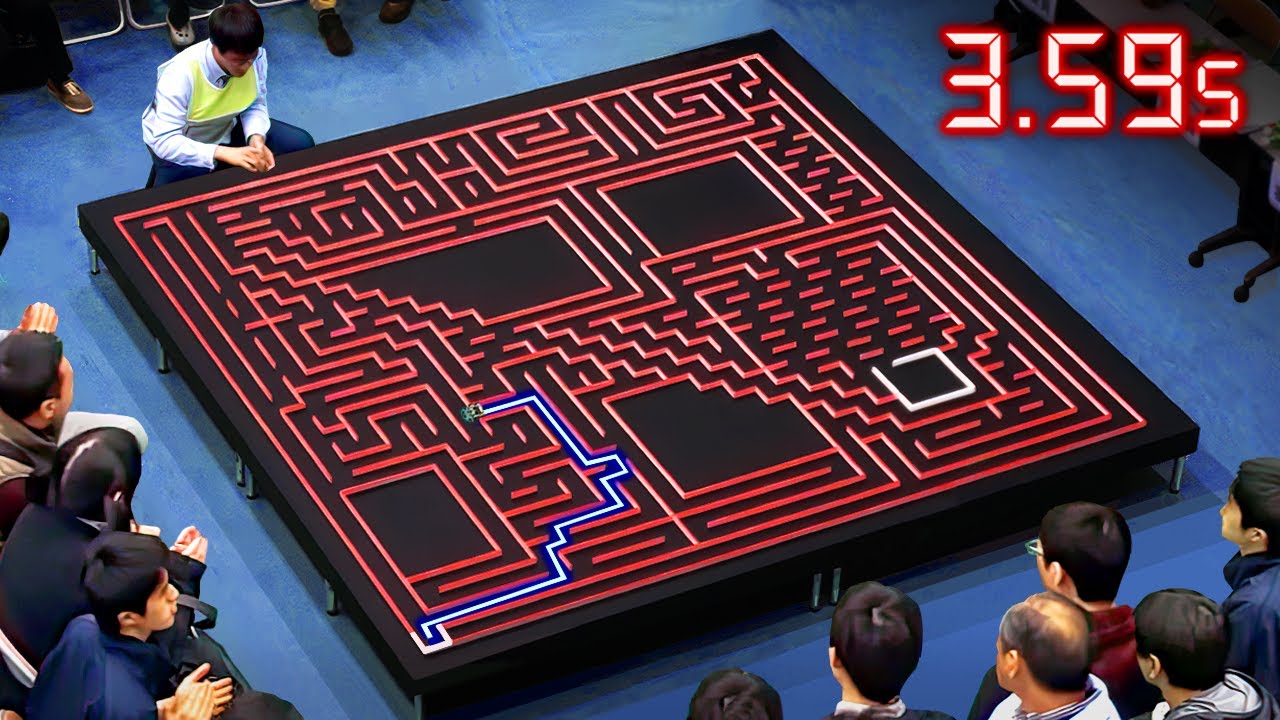
25:22
Micromouse: The Fastest Maze-Solving Robots on Earth
@veritasium
23.5M views•2023-05-24
Related Study Plans & Knowledge Roadmaps
Structured learning paths in Robotics
robotics
Building Delta Robots: Kinematics & Pico
01Foundations of Delta Robots & Mechanical Design
02Electronics and Microcontroller Setup with Pi Pico
03Delta Robot Kinematics and Coordinate Math
+ 3 more learning modules
65h6 modules
Explore Roadmap
robotics
Building Ballbots: Dynamics, Kalman & LQR
01Embedded Electronics & Omniwheel Actuation
02Ballbot Kinematics & Rigid Body Dynamics
03IMU Sensors & Kalman Filter State Estimation
+ 2 more learning modules
42h5 modules
Explore Roadmap
robotics
Micromouse: Hardware, PID Control & Flood-Fill
01Electronics & Teensy Microcontroller Basics
02Sensors and Actuators: Motors, Encoders & IR
03Precision Movement: Implementing PID Control
+ 2 more learning modules
35h5 modules
Explore Roadmap
robotics
CDPR: Kinematics, Arduino & Winch Control
01Foundations of Arduino & Basic Electronics
02Stepper Motors and Winch Mechanics
03Kinematics of 2D Cable-Driven Robots
+ 2 more learning modules
28h5 modules
Explore Roadmap