



















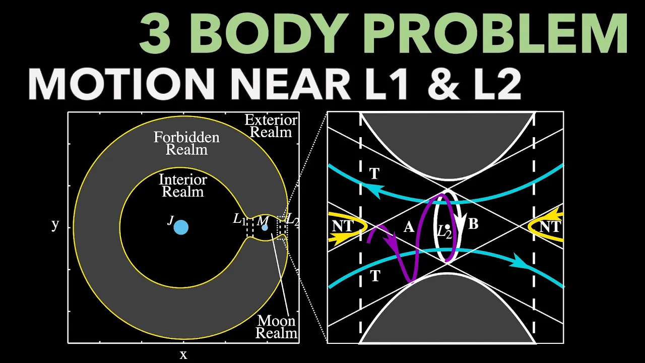


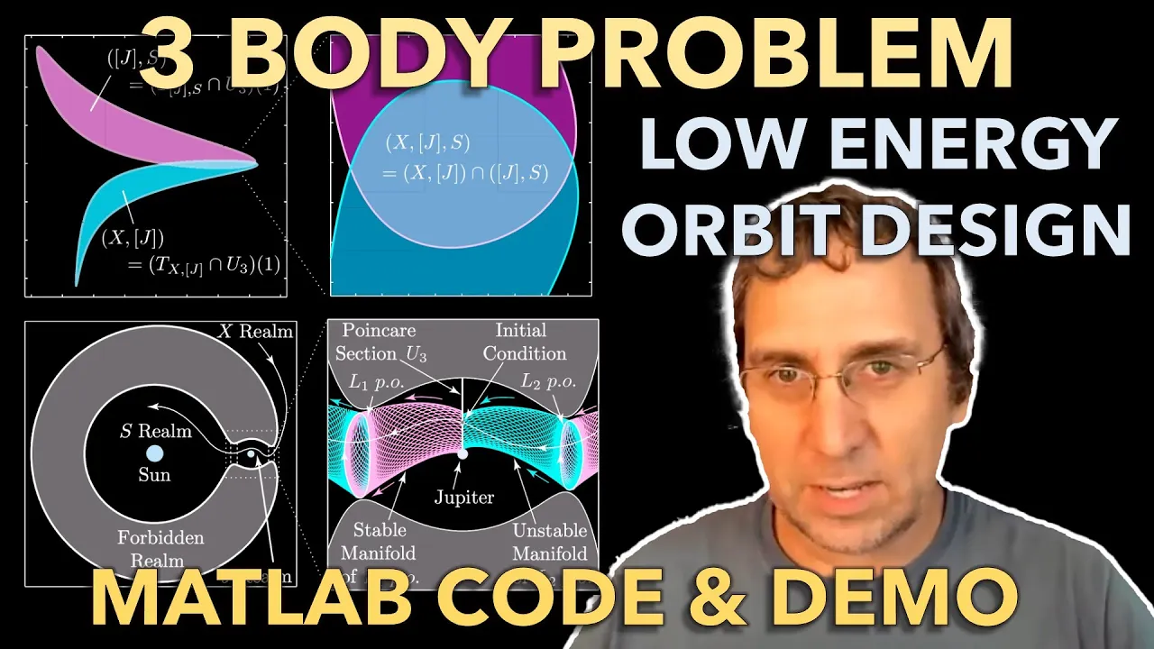
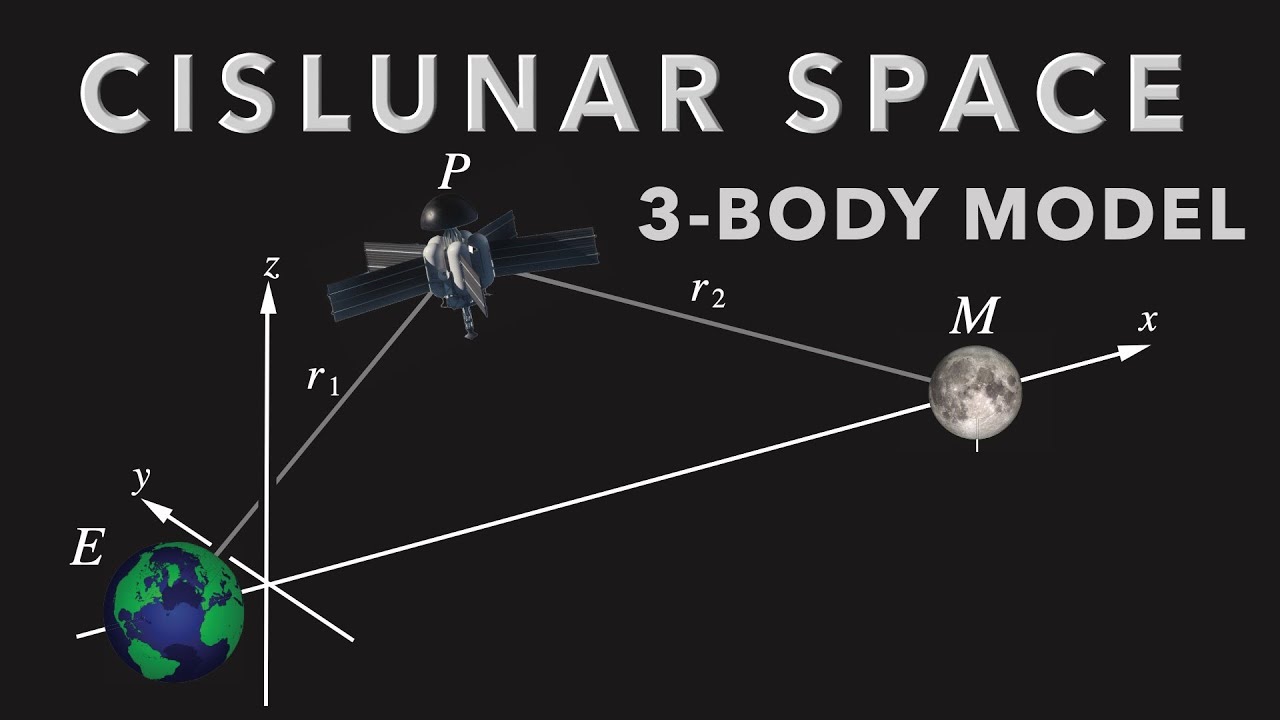
The Circular Restricted Three-Body Problem (CR3BP) equations of motion are derived by transforming from an inertial frame to a rotating frame that co-orbits with the two primaries, eliminating explicit time dependence and yielding autonomous ordinary differential equations; the resulting equations are: x'' - 2y' - x = - (1-μ)(x + μ)/r₁³ + μ(x - (1-μ))/r₂³, y'' + 2x' - y = - (1-μ)y/r₁³ - μy/r₂³, z'' + z = - (1-μ)z/r₁³ - μz/r₂³, where r₁² = (x + μ)² + y² + z² and r₂² = (x - (1-μ))² + y² + z², with the mass parameter μ being the only factor determining the type of motion possible for the spacecraft.
Rotating Frame Equations in the CR3BP: Derivation | Topic 3
Added:Newtonian mechanics and the formulation of equations of motion in inertial reference frames.
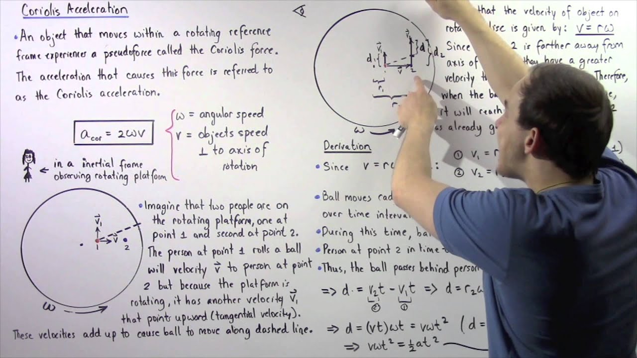
Kinematics in rotating coordinate systems, specifically the derivation of Coriolis and centrifugal acceleration terms.
The fundamental assumptions of the Restricted Three-Body Problem, where the mass of the third body is negligible compared to the two primaries.
Vector calculus and Ordinary Differential Equations (ODEs), including state-space representation and coordinate transformations.
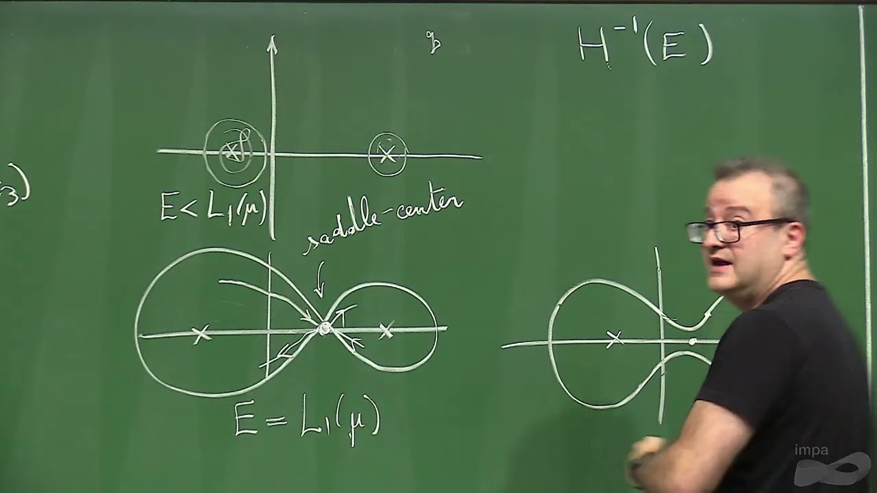
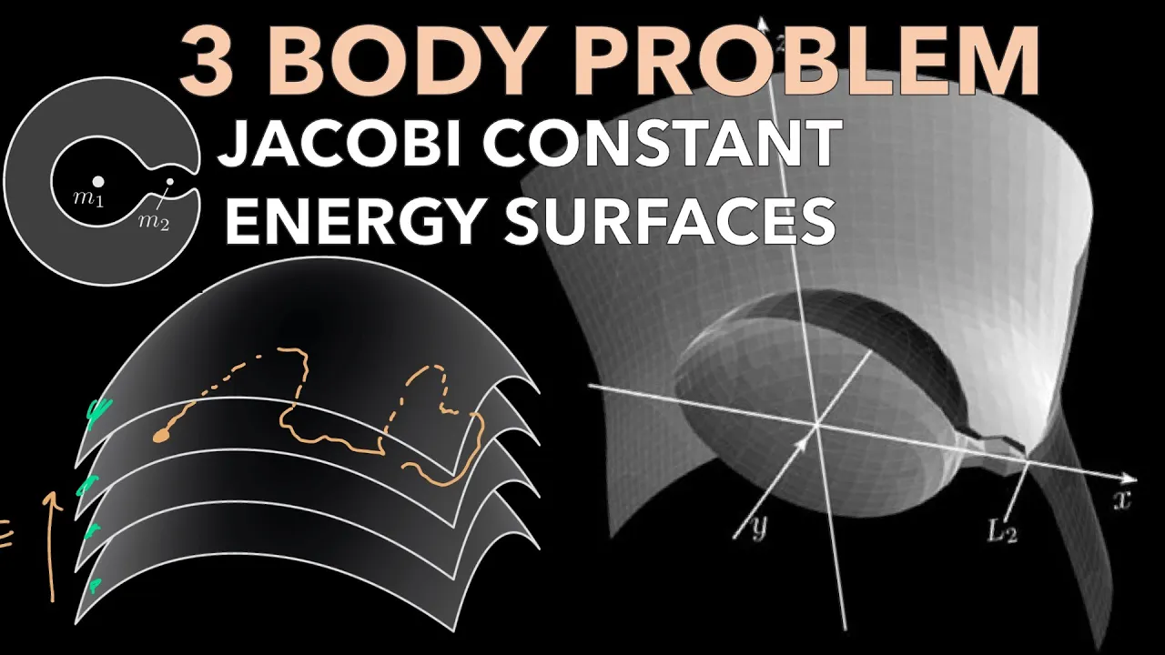
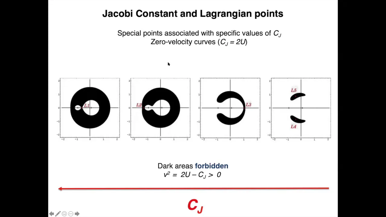
Derivation of the Jacobi Constant (the invariant energy integral of the CR3BP) and defining Zero-Velocity Curves.
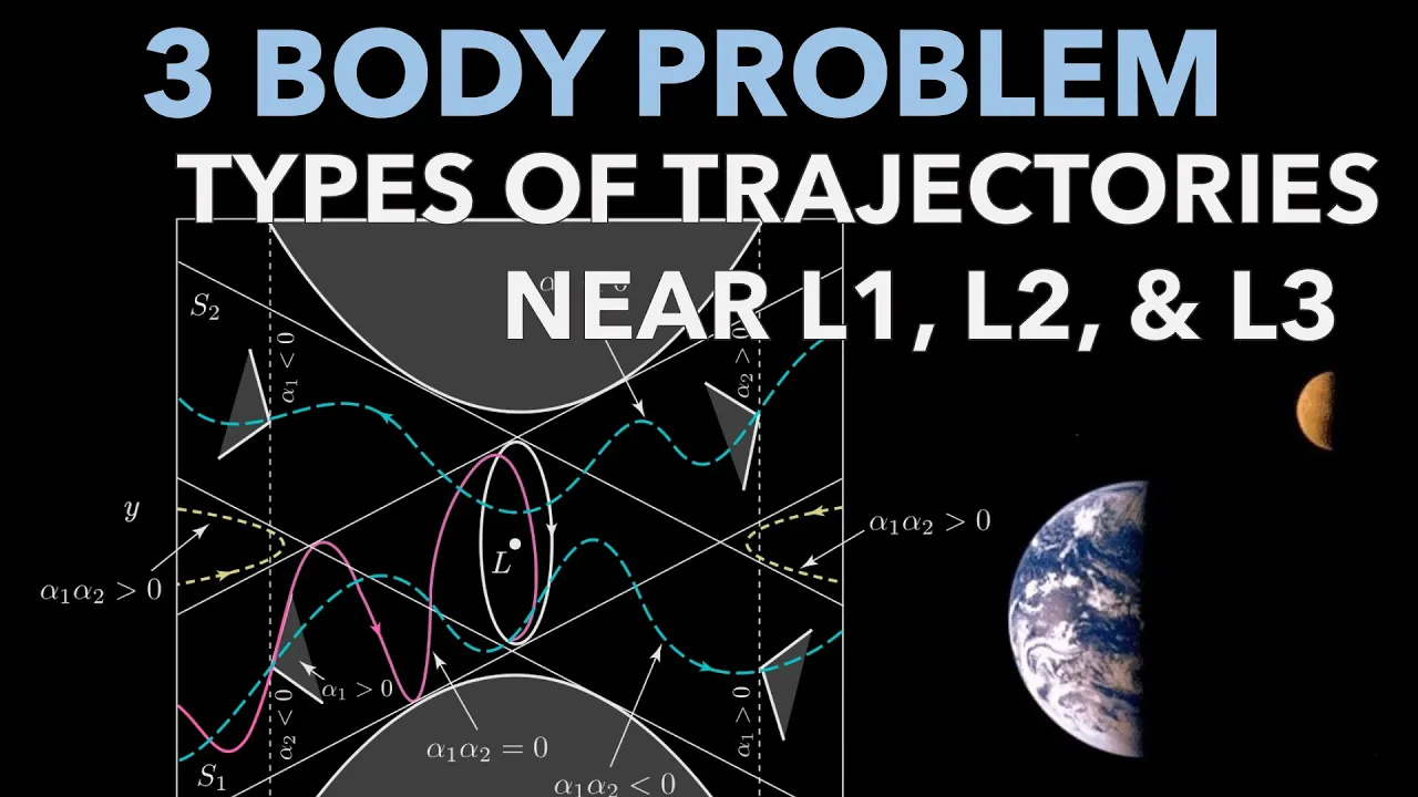
Locating the five Lagrangian equilibrium points (L1 through L5) and analyzing their linear stability.
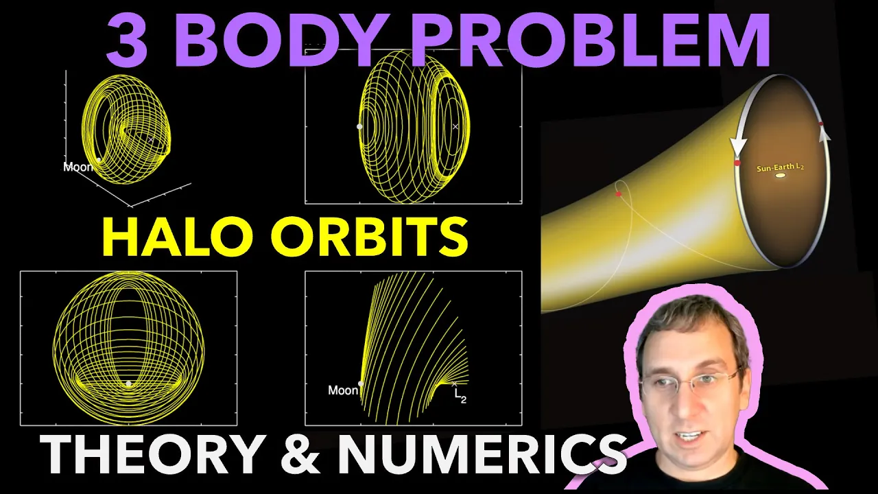
Computation and visualization of periodic orbits in the vicinity of Lagrange points, such as Halo and Lyapunov orbits.
Utilizing stable and unstable invariant manifolds for practical space mission design, such as low-energy transfer trajectories.
5.5K views116likes25:13Original Release: 2022-06-15
So last time we looked at the equations of motion derived using the Newtonian method and wrote it in a non-dimensional form. So if you remember, we used as the unit of length the distance between the two primaries m1 and m2. That's a natural unit of distance. And then the unit of time we introduced: this non-dimensional time tau. And one unit of tau is worth T over 2 pi of time where T is the period of the primaries. So if we're talking about a spacecraft in the Sun-Earth system the mu would be something like three times ten to the negative six, the unit of length would be 1 AU, so about 150 million kilometers, and the unit of time would be T over 2 pi where T is one year. So you can scale as appropriate for the system you're interested in.
But it's always easier to try to non-dimensionalize as much as you can. So we've in some sense did that so now we've got these non-dimensional ODEs so xi is the non-dimensional x direction in the inertial frame eta is the non-dimensional y and then zeta non-dimensional z so these are the equations of motion they're second order in the inertial frame so this isn't the usual way that people view and solve or you know generally just deal with three-body problem they usually look in a rotating frame so that's what we're gonna do we're starting from here but we're going to go further in some sense we've got vector differential equation here and we'll introduce a rotating frame. But first, what do I mean by the vector that we already have?
So we've got r written in the inertial frame and it's all non-dimensionalized now. Xi, eta, zeta. And the left-hand side up here looks like it's this vector and then we took two derivatives. Two derivatives with respect to the non-dimensional time. What we're going to want to do is get rid of these terms that have the cosine and sines. This time dependence is somewhat of a problem because that means every initial condition you give will also be connected to an initial time.
So it's just... It's easier to analyze a set of differential equations if you can eliminate any explicit time dependence on the right hand side. And here we have explicit time dependence.
So we'd like to get rid of it. It might not be clear exactly how but we're going to go into the frame that's co-orbiting with the two masses. And since they're moving in circular motion, it's a steady rotation so it's a rotating frame. The m1 m2 line defines a new x-axis and the out-of-plane direction provides the axis of rotation and the angular rate at least in these units is just one so this is the second derivative that the left hand side is. Xi second derivative, eta second derivative, and zeta second derivative. There's this thing we could do. If you've looked at the geometry of rotating frames, then hopefully this will be somewhat familiar to you. The N frame we could write this as being [NB] times the same thing in the B frame. So what am I doing here? I'm saying there's an inertial frame and now I'll draw it from above: n1, n2,, n3 forms a right-handed coordinate system. And we've got another frame. These are just unit vectors. And I'm following the convention that I tend to use when I teach rigid body dynamics. As part of that I also introduce the transport theorem and rotating frames. I don't think I'm going to use the transport theorem here.
So we've got two frames they've got a common origin and the angle between the two usually we would call that an angle theta, but now we'll say that angle is actually the non-dimensional time tau. So we've got two frames and the way that you would relate the B frame or what we would say is the rotating frame with respect to the N frame, this is the direction cosine matrix. I'm using what's called explicit frame notation. So this is cosine tau sine tau negative sine tau cosine tau. We're just doing a right-handed rotation about the z-axis or the number three axis. And you usually write it in terms of B with respect to N, the way I've done it here.
I know up here I wrote [NB]. We'll get to that. There is a frame and i can go ahead and put in right we've got m2 and then m1 and that forms the b1 axis the two frames if you wrote the b unit vectors as if they were a column vector we're just sort of grouping them for mathematical convenience this equals the bn matrix times n one and two and three so the direction cosine matrix completely describes how the two frames are related it also describes how two vectors are related so if you had a vector in one frame and you wanted to compare it to a vector in another frame so i could use any kind of vector maybe i'll write it orange over here if i had any kind of vector so i'm writing v just for vector this doesn't mean it's the velocity but any kind of vector if you have the vector you could write it in terms of b frame components or n frame components and they're related in the same way that the b unit vectors and the n unit vectors are related the vector written in the b frame components is going to equal b n times the same vector written in the end frame components if you haven't seen it written this way this is the form that i'm adopting and because we're talking about rotating matrices this nb up here this is the same as b and transpose the inverse of a rotation is the transpose of that matrix so i've got r written in the end frame is nb times r written in the b frame so instead of maybe this this vector here if i was thinking of the position of point p let's just call that vector r and we could write that position vector in either the b frame components or end frame components and that's all we're talking about here so um if instead of v i put position vector then that's what we got so when you take the inverse of this you get the equation that i already wrote up above n b and for convenience and to follow the notation that i use in my book i'm going to call this matrix a sub tau so a sub tau is just the transpose and i won't use the bracket notation anymore for a matrix so this is cosine tau and then now the negative sign goes up here negative sine tau sine tau cosine tau now notice that a sub tau depends on time what i'm going to want to do is take two derivatives of this equation so if i take two time derivatives and remember it's derivatives with respect to the time tau what do i get we'll get r n let's just start with one derivative this is a tau times b r and i'm going to take the derivative of that i guess i haven't said it yet so let me see what i'm using for the frames here in the rotating frame let me put the unit vectors b1 b2 and then b3 if we were to jump on that frame that's moving with the two masses then m1 and m2 will be along the x-axis and i may as well just call out the x-axis and then this one b2 is the y-axis and b3 that's the z-axis so i'm using lowercase x y and z to represent the position here's the particle p and from the very center of the system this is the position in the b frame so we're going to write that as x y and z so if we take the derivative over here on this right hand side so looking back at this equation well we could use the product rule here so we get a tau the derivative of that with respect to time times the position in the b frame plus a tau times the time derivative of that so that equation holds true if you work out what it gives a tau prime equals you can work out that it equals negative a tau times a certain matrix that looks like 0 1 0 negative one zero zero zero zero zero and this is times rb means we'll just put in what rb is x y z plus a tau and then that derivative which gives us x prime y prime c prime we can combine these two we could pull out an overall matrix a tau we have x prime minus y y prime plus x and z prime we could repeat this take the derivative of that and just see what we get so remember what this was this was the the left-hand side here says chi prime a to prime and zeta prime take the time derivative of that and we'll get chi double prime beta double prime theta double prime equals and you could use the same sort of procedure as before which you end up getting is a tau and if we group all these terms we get x double prime minus two y prime minus x y double prime plus 2 x prime minus y zeta double prime so we've taken the left-hand side of our ode for the motion of the particle and now we've written it in terms of similar quantities but in the rotating frame with an a tau out in front this rotation matrix we'll deal with that rotation matrix later what i wanted to point out is what we just did is get the left-hand side up here of the odes so now we want to get the right-hand side of the odes but written in terms of this rotating frame can we do that yeah so let's just look at the first term up here we'll look at this first od e and then hopefully you'll be able to pick up the pattern so we're going to try to write the right hand side but in terms of rotating frame components so this we might say this is the left-hand side now work on the right-hand side and let's start with the first thing so we had right chi double dot equals i should probably just repeat what i had up above so hold on what was it yeah okay it's negative 1 minus mu chi plus mu cosine tau over distance to the first primary cubed this was minus mu chi minus 1 minus mu cosine tau over rho two distance to the second primary cubed okay so let's try to write this right hand side using the rotating frame components i'll just give it to you here this is negative 1 minus mu that that doesn't change but what is chi chi equals x cosine tau minus y sine tau and then we put in plus mu cosine tau so that's just the first term about the second term this would be negative mu and chi again is x cosine tau minus y sine tau and let me write out this in terms of this will be plus mu cosine tau minus cosine tau all over rho 2 raised to the third now i'm using the same symbol for rho following what the book does i might just write this as r but that the distance doesn't change and so the distance cubed doesn't change distances don't change under rotation so what do we mean by this maybe i'll put it down here somewhere r1 squared equals this is now the distance to the body but in the rotating frame so if this is m1 this is m2 got x and y then the distance to the particle this is located at negative mu zero zero m two is located at one minus mu zero zero so they're just along the x axis so what is r one squared this is going to be x minus minus mu or x plus mu squared plus y squared plus z squared it's just the distance but as measured in terms of the rotating frame r2 squared equals x minus 1 minus mu squared plus y squared plus z squared we could write the distances there's no sines and cosines out in front of that but let's finish up what we have up here i'm going to pull out cosine and negative sine so i pull out everything that's got cosine tau times negative 1 minus mu x plus mu and then divided by r1 cubed then we have plus minus sine tau times negative 1 minus mu y and then divided by r1 cubed and then we'll have plus cosine tau i'm now moving to the second term here so we'll have minus mu x minus minus 1 minus mu over r 2 cubed maybe you can see where this is going plus negative sine tau this is time minus mu y over r 2 cubed move that over so just looking at this right hand side we could we hopefully you could see we've got cosines and negative sines if we do the same thing for eta double prime and zeta double prime we'll actually see a pattern and so this is what the pattern is chi double dot ada double dot theta double dot equals and there's an overall rotation matrix a sub tau that i could bring out and it multiplies minus 1 minus mu x plus mu minus mu x minus 1 minus mu all over r 2 cubed is just 1 over r 1 cubed similarly for the other two minus 1 minus mu y over r 1 cubed minus mu y over r two cubed and then similarly for the z it's minus one minus mu z r one cubed minus mu c r 2 cubed and that's just a vector but remember how we were able to write the left-hand side here it also had an a tau so if i just put in what we had for the left hand side this was a tau times x prime prime minus 2 y prime minus x y prime prime plus 2 x prime minus y and then z prime prime so if you want at this point the rotation matrices cancel or you just you multiply by a tau transpose to both sides and so what you get is you can get rid of all this and that's our ode written in the rotating frame so there's a written in terms of three scalar odes i mean it takes some work to try to get things in the rotating frame that was using the newtonian approach so this is the main set of odes that we're going to look at this is the restricted circular restricted 3 body problem equations of motion in the rotating frame and it's also already been non-dimensionalized that's nice dr ross you went from using the rows and then you went to the r's and then you went to the r's and the rows again and then in the final equations there you went back to the r's r is just the same as rho now i'm using little r's as if they're the non-dimensional distances my book uses that it's sort of the standard convention but this is going to be what i mean by the little r's it's the non-dimensional distance from of the particle from each of the two primary masses another thing that i'm going to do i'm going to not use this prime notation i'm going to use over dots for time derivatives because it's just a lot easier so from now on i'm replacing the primes with over dots but it means derivative with respect to the non-dimensional time so this is the form of the equations it's sort of a standard form that most people use some people have the situation where they have m1 on the right-hand side but nasa uses this convention so let's just stick with nasa's convention it's also what my book uses so it makes life easier for me and dr ross i have a question a little earlier you mentioned um transport theorem but then you didn't have to use transport theorem and this derivation presumably because this is in an inertial frame am i correct in saying that i just did everything in the inertial frame and then used rotating matrices to put it into a rotating frame so then it just becomes a lot of algebra so you didn't have to use transport theorem but you still took into account the fact that if dynamics were not in the rotating frame is that correct to do f equals m a you have to write that in an inertial frame but you could always view the resulting equations of motion in any frame you want translating or rotating even with unsteady rotation here it just so happened a nice choice of frame is a rotating frame and it simplifies things okay thank you yeah the key thing is the right hand side doesn't depend on time so that means you can simulate things and it doesn't matter like what the initial phase is all that matters is where the point p is with respect to the two primary masses and what the velocity is in that rotating frame so this is this is non-dimensionalized and the odes do not explicitly depend on time in the language of differential equations that means that these are autonomous odes because they're autonomous odes there's a lot of techniques from the theory of dynamical systems that can be used when you have time-dependent odes and what's an example of that the way that a cloud moves under the wind the wind is changing in time in fact in ways that are hard to predict so it'd be like having a right hand side or how the cloud moves that explicitly depends on time in a complicated way we don't have that so that's an advantage here i have written this in second order form and often it's written in a first order form in fact to simulate or matlab you always have to write things in first order form if you haven't seen it done the way that you put things in first order form let's just do it here you introduce variables we introduce something that we'll call v sub x and that's just the non-dimensional x velocity we're defining this to be x dot v sub y that's the non-dimensional y velocity v sub z that's the non-dimensional z velocity these three lines mean that i'm defining it that way but then these also end up being the first three odes so instead of having three second order odes we're going to have six first order odes in first order form this becomes x dot equals v x y dot equals v sub y z dot equals v z those are the first three and the next three are v x dot so v x dot is actually x double dot so i'm going to rewrite the first equation up there and what will happen we'll get 2 y dot instead of y dot i write this as b y plus x and then all that other stuff 1 minus mu x plus mu over r 1 cubed minus mu x minus 1 minus mu r 2 cubed moving on to the next one v y dot this will equal negative 2 it's negative 2 x dot instead of x dot i write the x and then this is plus y and then the terms that come from gravity 1 minus mu y for r 1 cubed minus mu y r 2 cubed z is always the easiest one because the two bodies are in the x y plane there's something about the x y plane that's special and in fact usually i'll be talking about the planar circular restricted three body problem where you just set z equal to zero and then everything happens in that xy plane that's where most of the interesting dynamics happens anyway so this will just be there's no weird vx and vy terms on the right-hand side here it's just the gravity stuff negative one minus mu z r one cubed minus mu z r two cubed so that's writing it in first order form you would give this an initial condition x at time zero y at time zero z at time zero v x at time zero the y times zero and v z times zero and then you would numerically integrate meaning numerically solved using something like ode45 i mean that's one of the things about the three-body problem is it does not admit general closed-form solution so that famously discouraged newton there's no analytical solution like there was for the two body problem so he left it for later mechanisms to try to work some things out so i this is putting it in first order form after deriving using the newtonian approach i would like to show you the lagrangian approach and i think the hamiltonian approach partly just to show their power the lagrangian approach is really cool and it gets the equation of motion so quickly your head will spin so we spent about a lecture and a half talking about the newtonian approach but there's a lagrangian approach if you appreciated this video please like and subscribe or just wait and watch the next video in the series
Up Next

15:01
Lagrangian Points Explained: Physics of Orbital Mechanics
@dcaulf
113.4K views•2012-11-28

12:53
21cm Hyperfine Transition in Neutral Hydrogen: Radio Astronomy Basics
@AaronRobertParsons
12.4K views•2011-10-13

32:32
NMR Spin Physics I: Zeeman Effect, Resonance Condition & Larmor Frequency
@nptel-indianinstituteofsci8064
2.3K views•2024-01-17

27:14
Entropy and the Second Law of Thermodynamics Explained
@veritasium
27.5M views•2023-07-01
Related Study Plans & Knowledge Roadmaps
Structured learning paths in Physics
physics
Nuclear Physics (Decay, Fission & Reactors)
01Atomic Structure and the Binding Force
02Radioactive Decay and Half-Life
03Nuclear Fission Mechanics and Chain Reactions
+ 2 more learning modules
12h5 modules
Explore Roadmap
physics
Soft Matter (Polymers, Colloids & Rheology)
01Foundations of Soft Matter & Thermal Forces
02Polymer Physics and Macromolecules
03Colloids, Surfactants, and Self-Assembly
+ 2 more learning modules
38h5 modules
Explore Roadmap
physics
Analytical Mechanics: Lagrangian & Hamiltonian
01Mathematical Foundations: Calculus of Variations
02From Newtonian Mechanics to Constraint Dynamics
03The Principle of Least Action & Lagrangian Mechanics
+ 3 more learning modules
28h6 modules
Explore Roadmap
physics
General Relativity (Spacetime & Cosmology)
01Foundations of Relativity: Special Relativity
02The Geometry of Spacetime: Equivalence Principle & Curvature
03Einstein's Field Equations: The Mathematics of Gravity
+ 2 more learning modules
55h5 modules
Explore Roadmap