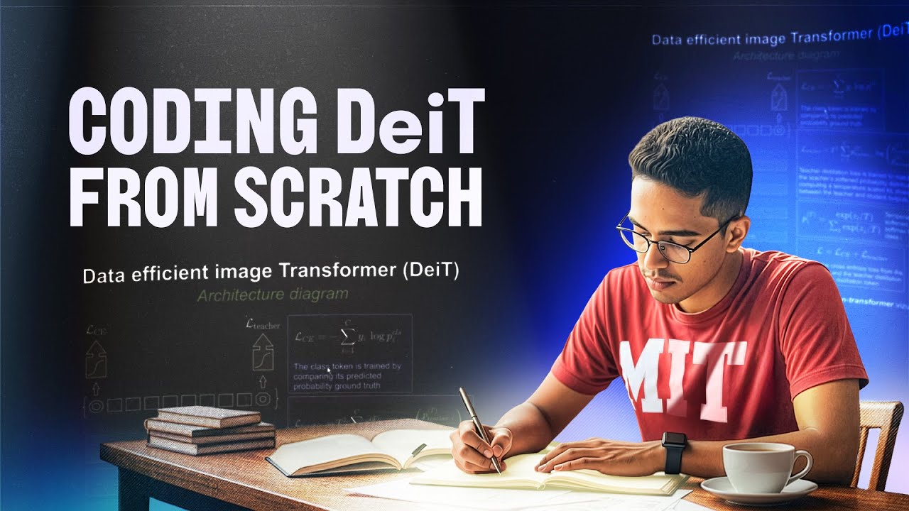
EfficientML.ai Lecture 16: Diffusion Models & Acceleration (MIT 6.5940) 59 chars

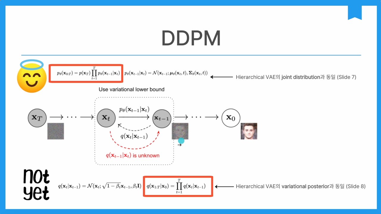
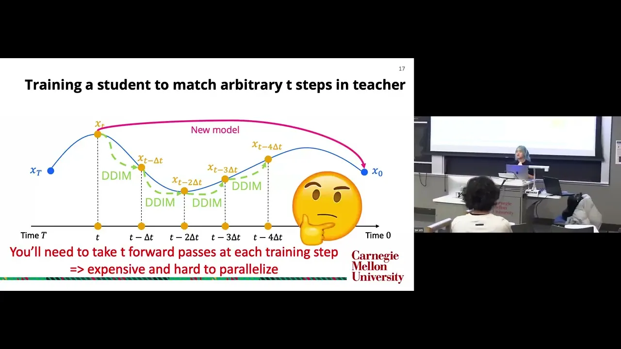
[00:00:01]all right good afternoon welcome to efficient ml. uh lecture 16 today we are going to introduce diffusion models and how to accelerate diffusion models with Advanced Techniques uh so in the last lecture G introduced The Deep generative learning so we first a sample from a data distribution to obtain a network and later we after tring uh this Network we can use the network to predict new images new contents so that's generative learning comparing this kind of discrimin model versus generative model a discrimin model gave a input and trying to classify it trying to predict the bonding box trying to predict the pixels the sentiment so we are given text or input trying to predict its attributes so trying to make a decision boundary on the other side the generative model is giving a label giving a class giving a condition the text we try to generate the content the image the text so uh trying to model to learn the probability distribution of the data so there are lots of popular applications uh using the techniques that we are going to learn in this lecture such as Adobe firly the mid journey. 3 for those content generation so a lot of comp applications by using the diffusion models so there is a pretty wide range of deep generative learning approaches uh so today we are going to focus on the diffusion models and this is the agenda for today's lecture we'll start with the basics of diffusion models uh introducing the denoising diffusion models and also how to add condition to the diffusion model latent diffusion models U how to use it to addit the image and also personalize the model and then we are going to talk about acceleration techniques how to reduce the number of steps by using fast sampling techniques like DD IM and also by using Progressive distillation to get fewer number of steps and also using guided distillation um to reduce the number forward forward um uh feed forward iterations and also those acceleration techniques by using sparcity and by using quantization to accelerate diffusion models we're going to see some domain specific techniques although recall sparity and quantization they're actually quite different some unique techniques in this domain specific setting so let's start with the denoising diffusion models basics there two concepts so um the denois and diffusion probalistic models so for ddpm basically had consists of two processes so the first process is the forward diffusion process when we are gradually adding noise to the input the input gets more and more noisy and there's also the reverse path this reverse diff diffusion process is generating the image from the noise it starts with the noise and then gradually Den noise um to generate the data by D noising compared with Gan models which we learned from the last lecture uh this kind of forward process defines a iterative pro mapping process not just one time but iterative M mapping from data distribution to a gshi now noise and this backward pass learns to reverse the forward process uh step by step so learn very fine um grain those details step by step rather than again you just do it once so this is some illustration about the forward process and also the reverse process in the fold process uh we can see we destroyed the data original image we destroy the data by gradually adding um small amounts of noise so starting with clean image and in the end it becomes ging noise compared with that we have the reverse process starting with noise and gradually denoise to create data by gradually denoising um a noisy code from a stationary distribution so starting with pure noise and then with d noise to get original to get a Target desired image so in this forward process we can model the relationship between XT and XT minus one as a gotion distribution so the mean this is the mean this is the variance so beta is a predefined constant to control the diffusion speed which is only related to T and it's linear really linearly growing with the time stamp gradually adding more and more noise uh to the uh to the input image so this is the relationship between adjacent two steps XT minus one and also XT okay what's the condition of XT minus one to get XT but how do we sample XT directly from x0 okay from x0 to XT so we can do a little bit of math don't be afraid of it I walk you through so here we plug in the equation this the mean this is a variance okay this is following a uh ging distribution here the relationship between XT minus one and XT is like this these are constants beta is only related to T we can do a little um transformation Define Alpha t equal to one minus beta T so we can transform the relationship into the second row and then we can plug in XT minus one using a similar form okay the relationship between XT - one and XT minus 2 can use similar form of equation so that we can get relationship between XT minus 2 and also XT and here is Epsilon T minus 2 is also following a gan distribution so now we have two Gan distributions Epsilon T minus one and also Epsilon T minus 2 so adding two gion distributions basically um the variance we are adding the variance together and square it and so that we can merge these two terms together into a single term and we put a bar here to distinguish them okay so we have a single ging term here and beginning term stays the same we can repeat this process on and so on until we reach x0 okay so it's it process from XT to XT minus one to XT minus 2 and all the way to x0 okay and you have a chain of alpha T Alpha T minus one all the way to Alpha 1 together with a G distribution here we Define a new term uh for this combination this Alpha multiply them together we denoted as Alpha T Bar then we can plug simplify the writing of the relationship between XT and xt0 is like this so that we can get a relationship from x0 directly to XT okay it's a normal distribution this is the mean this is the variance so we can uh directly get from zero to a certain time stamp and just rely on these two definitions Alpha T and ARA T bar so that we can get this repeating the equation from the previous Slide the relationship between xt0 and also XT as this is the mean and this is the variance we call it a diffusion kernel this is what Alpha T bar looks like T goes on it's gradually a diminish to zero so for the sampling process X we know X zero so we can get XT this is the relationship and here we are having a um normal distribution in the back and beta T is designed such that Alpha T is close to zero when um um and also the relationship between um um Q x0 XT is following the normal distribution so X Alpha T when it's getting T is getting large is close to zero so let's now see the reverse process the reverse Den noising process from XT all the way to xt0 has to assume when beta T is small the relationship between X XT minus one is also a g so that we can write it in this format this is the mean this is the variance the me Theta XT is the mean which we are going to predict and it's learnable actually that's where the essence of this class so and here we defined Sigma T Sigma T Square to be equal to Beta T there a little bit of math but we'll go go to the relative quickly since we are focusing on the engineering aspect so um this is the loss we're trying to define the loss so that we learn how to how to train it so uh this is the minus log p i0 x0 is the real data we want to maximize this log log likelihood by using this evidence lower Bond we can find the bond with which we are going to not going to put them in this lecture uh by using this is basically The Joint distribution from x0 all the way to XT and this is our loss function we are trying to minimize a meting some linear algebra we can simplify that into three terms uh since here uh this equation is parameterized by Theta the first term is not related to Theta so we only focus on the second and third term for the relationship between XT Z and also XT minus one we can use conditional probability to simplify it in this way okay so this is the G the other term we have seen before from T to T minus one is also a ging okay so both of them are ging so that we can further simplify that and this first uh this first term um is can simplify them in a similar manner so let's first try to simplify the middle term and soon we are going to see how to map this into py torch language if not comfortable with the math don't worry about it at all I me some linear Al some algebra the loss function is basically this Square this Square term and trying to minim minimize this Square term we want to make this mu Theta XT equal to this big term so that you have the square that is minimized notice this ulon is the noise the added noise is only the only unknown so that's the goal our neuron network is going to predict okay so Epsilon Theta Theta is the parameter of the U net is trying to predict the added noise so all we are doing by Deep learning is trying to predict the noise and predict the noise given the input given a noisy image we try to predict Noise Okay and we subtract the image subtract the noise from this image okay and then we trying to get this new Theta so that we can plug in this mu Theta back into this equation and assuming this relationship from x0 to XT um during the forward proc forward the process we can plug it in to simplify it in this way okay LT minus minus one can be simplified in this way so this L Zer which is right here also have a very similar form so now we get a relationship okay given the image uh we try to predict the noise using Epsilon Theta epon Theta is the unit where bu the bul of the computation is spent okay and we uh try to predict the the noise and use that as the Lost term so writing that again uh we uniformly sample from one to T and also sample a um correct image Target image and also sample AI noise and this is the ground truth noise we are trying to predict and this is the function the unet um we are trying to uh apply a neuron Network given the input we are trying to predict the noise and this is basically XT the input by calculated by the diffusion kernel using x0 so we simply set Lambda tal to for better um perceptual quality and so far lots of math but everything can be condensed into a very intuitive image and this is what I want you to remember not the math equations but this intuitive picture let's walk them through carefully so given x0 okay and multiply with a constant term this is what rpha T looks like with T is getting smaller and smaller um and this is a random noise random go noise multiplied with one minus this term okay and then you add them together you have a noisy image can still tell it's a cat but it's added a lot of noise and you pass this through a unit okay down sample and then up sample pass through this unit trying to predict the noise okay so all we are doing here everything unique in this lecture is that we are doing a pixel to to pixel pixelwise prediction given a noisy input original input noise noisy input given a noisy input trying to predict the noise how to predict it by matching that with the noise you added to the input image that how we closed the loop okay give it a noise input trying to predict the noise that was added to the image okay so we can make it a lot more easier to understand let's see the training algorithm so we uniformly sample a t from time one to time T and then we sample an input image such as a cat it can also be a dog as long as from your desired uh distribution and then we sample a negotiate Noise Okay and we um get XT following this equation this is the original input image okay original clear image and this is the the noise this is the noise and add them together we have XT add them together we have XT and we feed this XT to Epsilon Theta what is Epsilon Theta it's a unit Theta is the parameter be tens of millions of parameters this is Epsilon Theta okay we feeded with epon Theta and it's also Prim parameterized by T since during different time stamps can be different so we pass this XT through this unet and trying to predict a noise okay we are trying to predict a noise and we are trying to minimize the difference between the predicted noise versus the original noise and that's all we are doing as a loss function now that's all what the equation previously is about you want to predict the noise uh I don't know if that works right and these terms you have to be very careful that's all what the derivation is about yeah so this is the training algorithm and let's see what about at sampling time what do we do over there so let's again start with the intuitive image okay so we have a noisy uh noisy image we try to get a clean image and what do we do here again pass it through a unit okay and trying to predict the no noise and we subtract the noise of course there are certain terms right here those are just constant with with respect the T okay so this is Alpha T going down linearly this is Alpha T Bar multiplying them together close to zero in the end and this is uh Sigma T Square going to increasing so this is the these constant terms so the essence is that we are trying to subtract this noise from this noisy input okay the unit is predicting the noise we're subtracting the noise from the original noisy input and trying to get a d noised image but here interesting part here we also added another GOI noise and then this is it becomes the next time step txt minus one okay so this is XT um nois image XT minus one still a noisy image but less noisy just repeat this process until it it's completely clean image okay so this is a intuitive image I hope you can remember and on the right hand side you can naturally translate this into the algorithm okay so starting with XT which is completely a random noise and then from T to one we are doing the reverse process so this is from T to one we resample ging noise is here um and then we use XTX input Fe to the unet which is Epsilon Theta Theta is the parameter in our um in our unet use the UN to predict the noise and use XT to subtract the noise okay and that gets this term and finally we added the ging noise to get the next XT minus one from XT minus one we uh continue in the for Loop to predict XT minus two and until x0 so that's the denoised image we are going to return so that's the same thing where this equation is about um so you can remember the equation and also both the equation and also the intuitive uh illustration of this process so where is The Bu of the computation here it's the unit although area wise is small but actually most of the computation is going here it's a pixelwise prediction given noise input predict the noise have large resolution here then you have large resolution here okay so that's where the bulk of the Computing is going these are all like pixelwise subtraction okay pixel wise addition doesn't have a lot of computing all right so um using diffusion model these are some of the examples uh emerging as powerful generative models or performing G sometimes uh some cool images all right so what if we want to generate specific stuff like particular class or given a text to generate the image oh so there's a metric called uh FID people use that so previously we generate a lot of generated image versus real world image and measure the similarity with the pixel wise difference with the real world image and check out FID forer all right so it's about how do we add condition right if you use mid Journey you want to type into some some words to generate a moon generate something a horse riding a moon right so um how do we add those condition we call it condition okay so unconditional generation is basically uh using this term and if we uh compare with the conditional generation XT minus one not only depend on the previous XT but also depend on the c c is the condition okay um so here we have mu Theta not only as a function of XT but also as a function as this condition and that's the only difference so here the unit previously has only one input which is XT now it has a to the T but now it has another input as condition which is um the text or the image or the class label you input as a condition okay so this IO now has three Prim the image time stamp and also the condition so let's see um what what kind of condition types are there we can have a scalar condition like a class generate me some docs generate me some cats um class ID just a single scaler class ID we can also have pixelwise condition okay pixelwise condition like um so this should be actually um space this should be text condition there's a typo here this should be taex condition a sequence of Tex tokens like a photo of a moon gate g make sure you addit polish the slide to fix this should be tax condition on the on the slide okay this is what very widely used M Journey these days like you give a text uh description what you are trying to generate the next one is the pixelwise condition like giving a mask like a cat a mask of a cat or um a cany edge of a building so pixel wise condition so let's start with the scalar condition like a like a class ID okay so this is the original feature map and we want to add those class condition to the feature map so we pass it through a encoder so that we can get get a representation by batch size versus c c is number of um channels and we pass it through the MLP to match the number of channels to be the same as the feature map so here we have four channels the invent here should also have four channels so the C here matches with the c here and then we can do a broadcast ad okay broadcast this pixel to entire XY location similar for this pixel so to the second channel for the entire XY location so that we can get a conditional feature map this is simplest uh method to add a scalar condition a more improved version is basically uh double that okay we have not only um addition but also multiplication so we uh predict a scale and also a bias okay to scale the feature map and then add the bias that's why here we have multiplication and addition so that's how we insert the scaler class condition okay the next is the TX condition how is meid Journey handling the TX we input to the image so that's using a cool technique called cross attention Okay so we have the input feature we talk about viit we chop the image into several patches and each patch becomes a token so that's the that's the key Q that's the query and K and V are basically the text conditions like photo of a moon gate this is the text we did to meet Journey we treat them as K and V okay we use um um pass it through a w Matrix to transform it to get a feature as k pass it through the WV um to uh project it as the as the value and then we pass it through attention why we call it cross attention because some of them is coming from image some of them like K and V is coming from the text well Q is coming from the image and then we pick each patch each token from the image and to multiply with the K to get the similarity to get the attention and we use soft Max to make it some up to one and then we use that as the weight to get a weighted average of of the V of the value okay and this comes becomes a output token so we can repeat this process through all the uh input uh image tokens and to get a output image so this is how cross attention works by using um qose soft Max sum up to one reg scale it by by Dimension and then times B uh to get the um text information injected into the image okay so this text information injected into the image so finally the output token is a image token you put it back it becomes uh the um mingled text and image this is a very effective way to mingle the text with image by using cross attention okay so the last uh last type how to inject condition is by using this pixelwise condition so a very intuitive way for example we want to generate a cat that looks like in this position it looks like this so we can just put the segmentation map concatenated with the Noise Okay and then predict trying to predict the noise very simple just concatenate other so other better methods one of the represented one is the control net which got published in iccv uh one month ago very fresh very widely used technique uh it's actually pretty cool given input uh cany Edge this is default generated here can also input the text um the text condition like Masterpiece of fairy tale giant deer golden and and qu City GIC something so all the generated image looks like the um cany Edge input cany edge condition condition okay or we can input a human pose human pose again it's a pixel wise condition and make sure the generated uh men all follow this gure follow this poles okay can generate default hand is here exactly following uh the condition or Chef in kitchen or Lincoln Statue you can have not only the packs but also such uh pose condition and also cany Edge uh condition and they all look very similar in their pose and how is that achieved okay so um it's very interesting by using control net this before you have a neuron netor block um what we added here we fixed this original neuron nital block but make a copy okay make a trainable copy in neutralize the same way as the original neuronet block and we add a zero convolution before and after it's a bit misleading by talking about zero convolution in fact they are zero initialized one by one convolution so initially they are zero but after 20 they may not be zero why initially they are zero because as if you don't have this branch adding this zero Branch injecting the condition initially they're not injecting anything because they are initialized with zero so just using this main branch in the beginning but after training this convolution this convolution they are both one by one they're no longer zero so that they can inject the condition from the top that's the key idea from control net and we can stack multiple such blocks together so this is original unet okay down sample up sample so in the down sample phase we are going to add the control the control Branch okay so uh this is the could be the pixelwise conditions like the pose map can also be the semantic mask can also be the canny edge we show like the edge of the cany edge of the deer as a input image pixel wise okay uh we pass it through the zero convolution and this is the original condition we inject by cross attention like text prompt we have seen the Lincoln Statue text text prompt this is still using uh the cross attention to inject those text condition and then we copy the down sample stages from the original this is stable diffusions incoder block I'll copy them and then uh on the up sample stage they don't have any um they're directly using zero convolution to feed it back to the original up sample phase of the stable diffusions decoder so this is how this um pixelwise uh Maps either semantic Maps or can Edge or or pose those conditions are injected okay copy another Branch um initialized with a zero and this is copied this is initialized with a zero uh feed it combined with cross attention with the original text prompt and feed it back um to the original main branch okay throughout the training the main branch is fixed we don't touch the main branch but only this side branch to inject the condition okay so that's control net and now we want to talk about how do we treat diversity for Quality so we want to also generate um a specific um class okay so we talk about we can not only given the class we we can get a image but also we want to make it follow this particular class so we want to train classifier at the same time as the generator okay so we add not only the original gradient but also the classifiers gradient okay and then a new sample distribution is defined as this is just from this class to generate uh this this XT but also this XT should be predicted as this class and we put Omega uh as the strength to control the relationship the strength so this original sampling plus the classifier scad in to make sure the generated image will be classified as the original desired class and we have a guide guidance strength Omega on the top so if you put them in the log space this multiplication of these two terms becomes the the addition that's why we put Omega on the top because getting the log they become a a a a multiplier in the front Okay what we means to our diffusion equation is that basically we add another term another term to the um to the prediction okay so this is the original naive conditional sampling and we have condition T and XT and trying to subtract or predict the noise this is subtracting the noise um and get the next step okay and later we not only predict the the noise subtract the noise but also we add another term Trying to minimize the loss trying to make the classifier we can classify this XT as a desired class okay so that's the new classifier gradient that gets introduced to make sure um the generated image they all belong to the same class okay we want to encourage the loss such that the generated image is all predicted as the desired Class C in this case and actually it's pretty effective uh like if Omega is pretty small okay uh there are some dogs but not all of them look like dogs some of doesn't look like dog but if Omega is pretty large meaning that we want to make sure the loss of the classifier is pretty small so that all the generated image look like dog and actually looks like dog a lot what are the limitations here you TR classifier it can only do classification so it can only work on class condition but how about tax condition how about pixelized condition is not straightforward forward and also they need to train additional Network a classifier okay which is complicated so how do we solve this problem so let's look at rather than classifier guidance let's look at classifier free guidance okay so to support diverse condition class text or pixels okay no extra don't need to train any actra classifier network okay follows Spas rule given XT I want to predict the C and rewrite it in this way okay this is a conditional model this is unconditional model which hinted that now we want to forward the neural network twice one is a conditional model the other is unconditional model with c and without C want to double the flops later we are going to talk about how to reduce the compute over there um so if you expand our previous equation defining the classifier guidance remember there's Omega controlling the strength of the original floss versus the the new classifier introduced um function so we can further simplify that by by using base rule uh in this way okay we can see there are two terms okay uh in the log space if we um expand it it'll be this one subtracted by the second term here one is conditional the other is unconditional and one is condition on C the other is not condition on the C the and the uh here we have omega plus one and here we have omega then if we continue uh to derive um the equation for the classifier fre guidance we can compare that with the original conditional training is actually quite simple so during tring time we just sample the condition okay previously we have this uh this condition we always have this condition uh given x given T given C we try to predict the noise minimize the distance and now with probability uncondition okay we randomly drop the condition so that we can train it unconditionally so C here has some probability to be to be n adding no condition okay so that's the only change and C here is the same as the C here okay uh so that's the only change we s during sample we sample with some probability that the condition is none what about at simping inference time at inference time remember we have these two terms one is conditional the other is unconditional okay uh the constant here is Omega plus one here is Omega okay remember the term here Omega plus one and Omega so that's the only change we made here at inference time we have to write the inference twice okay uh combine the results of conditional and also unconditional forward process is doubling the flows we have to uh do the same um run the same network twice okay the network Theta epon Theta they are the same we have to run it twice and this is the result from no guidance versus with gu guidance okay um such large uh W usually lead to better quality but less diversity so the advantage of such classifier free guidance is that it can generate to any conditional form not just class uh since we don't need to train a classifier no need to train additional Network so this condition if you see the previous equation it can be U anything you can use um Tex Tex condition remember we talk about cross tension to inject the text condition okay and also we can use the pixelwise like a mask condition uh by using the control net okay so this is very simple just use with the condition so without the condition can be any method we have learned so far to inject the condition okay not necessarily relying on it has to be a class so this C can be any condition using the method we learn to inject the condition and the only catch here is that we have to forward the network twice all right so that's a lot of content let's take a five minute break before we jump into latent diffusion models all right welcome back let's continue the discussion so diffusion model seems pretty complicated math but all we want to remember is that what we are predicting we're predicting the Noise Okay so classification network is plus predicting a class um detection network is trying to predict the bonding box segmentation model is trying to predict the SE The Mask diffusion model is trying to predict the noise why do we need to predict the noise because then we can Den noise that's the essence of this diffusion model uh so let's continue to talk about the lat diffusion models so when we have a high resolution how do we generate a pretty high resolution image without incurring a lot of computes so uh we first pass through the image into a um R TN variational auto encoder to encode it into a latent space which has much smaller resolution like one quarter or one e of the resolution okay and we use um run the diffusion process in in the latent space and then we use the other half of the variational vi uh the decoder part of it to try to reconstruct the image okay so rather than um running the diffusion on the original pixel uh original pixel space we run it in the latent space so the advantage that applying to the lat spaces we can have simpler denois because the resolution the dimension is much smaller and also can lead to faster synthesis that's actually very widely used and algorithm wise is actually just one line of code here very simple we just pass the original input image into a incoder and get a latent space and we run the diffusion process in the latent space okay so we add a noise pass through the unet to predict the noise and try to minimize the loss the only difference is here we pass it through encoder to make it have a lower resolution similarly for the U sampling stage rather than directly get the output we pass it through a decoder to get the output everything before is exactly the same okay so we have the uh the noise we use the net to predict the noise subtract the noise from the original input we add the noise trying to get the next uh next time step and finally for Z z0 we pass it through a decoder to reconstruct the original input so this is widely used like stable diffusion XL they're using such latent diffusion method like astronaut in a jungle code color palette and also a deep CA diver floating these are high resolution images compared with the cats and dogs we' seen before the image resolution is much higher much higher quality they're all using such lat diffusion methods question certainly how do we edit it that's exactly the next part we are going to talk about how do we edit the image like we can draw something draw a tower draw some trees draw a bedroom draw some scenery okay and how do we uh use SD edit to actually get the corresponding picture cor um that that's associated with this hand stroke based editing so the idea is that we use our hand to draw something very naive like roughly a tower Some Cloud around it some Bas on the bottom um so you assume the image distribution is here our stroke is here uh there is some distance and we add some noise to perturb it with Some Noise Okay so the stroke becomes becomes noisy becomes noisy and the good part is that you can assume this is certain point in the diffusion process and then we can predict the noise from here and gradually remove that prediced noise remove the predictive noise and uh this Center this mean will shift from here and gradually shift toward the original image the real image distribution so it looks like a real image output you first add a noise and then predict the noise then subtract the noise that's the magic about how do we convert this stroke into the image so this stroke based editing uh we can also do image to image translation the original hand drawn picture and then this is a generated picture again we add a noise and then predict noise and then the noise so that we can shift the distribution ution from this hand drawing image to the desired Target style what about text based editing like here the boulevard are crowded today how can we T tone down this crowded make it less crowded lot of people here fewer number of people um a photo of a cat riding a bicycle and change it to a photo of a cat riding a car riding a car and then here here um this is just image and then we want to add a style children drawing of a castle next to a river immed turn the castle River into a children style or we can add some Jetty beans to the cake add some Jetty beans to the cake and this looks like magic and how is that achieved remember how did we inject the text pred by cross attention right what is cross attention reminder let's go through it again so the pixel Fe features we um uh chop it into uh different patches each patch is a token that becomes the query the que and the key and the V are both from the text for example here this is the the a prompt um sentence several prompt sentence and you get attention map attention map for each quer you get attention map so here since we have five uh text prompt tokens you get five uh channels in the attention map you multiply by the v v is from the text and then you get the target output what about we do some manipulation for the words like uh removing bicycle and change it with a car everything is everything else is the same so here we want to just use original um cross attention map from photo of of a car riding a bicycle so that the location of the bicycle is exactly Remains the Same so here up up to here everything is the same we just plug in the new V okay the V the last one of them is a car rather than a bicycle in this case so that the process tension map matters uh determines the location the location doesn't change only the thing only changed is the V so that original attention cross attention stay the same only use the new V from from bicycle to car what about this case adding jelly beans okay to the decorations adding some words okay so here we add a new uh phrase so the old words will use the original cross attention map from old to new and the new words use the new map okay so new words okay longer uh token number of tokens in the key so the attention map has more channels the V also has more so you have some couple of new attention Maps what about um weight getting different weight like uh tuning down the crowded make it less crowded or make it more crowded so we can simply re weting adjust the magnitude of a specific token like here you have five tokens then you have five channels in the attention map you want a particular to to tune up or tune down you can weigh it tune it up or tune it down for the certain corresponding Channel um in this way to tune it up or tune it down so that's how to edit the image how to personalize the image say want to draw a picture of this particular this is my or someone's lovely dog we just want to draw a particular dog in different places a CW place in a dog dog in a bucket sleeping swimming but everything is not the general dog but it's my dog it's a specific dog that should look like this the dream Booth is doing that which actually a challenging a challenging task for example given the input image which is a clock very unique clock three is written in this this way very artistic style but D to using the image guidance is not generating something exactly looking at M clock the three is in the is not the style I want um and also we want to change the background this is probably on the bad but also I put it in the te context of some green outside but this one is following the context but the fality is po three is in the middle it's not like three here um but by fine tuning we can generate the same clock okay in the background of several uh green Outdoors okay you can make it both m main the fality and also use new contacts and how is that achieved so Jo Booth basically fine tune the model OKAY the model takes um it's a text to input to image model okay so we have a couple of pair uh training data saying this is a dog this is the dog this is the dog and we put it to fine tune this model so that I can generate a a customized model OKAY generate a customized model no the original General text image but this is a personalized text to image just one model for one object then you have a dog you have a new TR a new model but later you want to say make an advertisement for for another stuff you have to tr find you another um personalized text image model okay so the input is just few images of a specific subject and the class name and the process is basically fine tune the text to image model to create a personalized personalized version of that particular subject and output is a new model OKAY capable of generating images of that subject in different contexts and the limitation is that you need one fine-tuned model it's only specific to one subject here like a personalized Model A V dog is in the beach in the beach a v dog is walking in colorful carpet colorful carpet another limitation for like M journey is that I cannot generate faces like we what we want like fa face riding a horse L doesn't look like f right but existing work either um need actual fine tuning right like the dream Booth you can find you need to fine tune the model which is costly as we learned or it can generate poor M person like Newton and Einstein we want them to sit in the park they get mingled together it looks like each other um or you our approach you can distinguish them rather than mingle together or overfit the reference image so like fa riding a horse just have fa but no horse but now we want to generate something like this if you're riding a horse how is that achieved looks like a bit complicated but let's walk you through that um a woman and a man are standing together so we first get the a picture taking a picture of the two two subjects and find a a segmentation mask this can be easily obtained using Auto annotation tools for example using Sam and then you give the text prompt pass it through the text encoder to get the texting beddings a woman and a man sitting standing together okay and you pass through the image into the image encoder like the clip image encoder and we concatenate since we know the man correspond to this image the woman corresponds to this image we concatenate the features from the text embedding with the subject embedding okay um and then we get a conditional embedding so blue oh sorry red and green or resp to red and green here and then we inject the conditional ined by cross the tension we learned using the unet okay so we fine tune the unet fine tune this projection F tune the encoder such that it can learn that we should match the cross attention map woman and man to be in this location rather than mingled together okay so we are trying to minimize the distance between the woman's cross attention map with woman's segmentation mask since we know woman should be here and the man should be here here okay so by using such cross attention localization we can solve this problem where people are in entangled together so at inference time again we have the text prompt pass it through the text encoder we get the tokens image through the image encoder we also get the tokens we add the corresponding man man into the uh text with the image and the trick here is we need to delayed subject in I condition so in the beginning okay this is in the beginning of the den noising step we only take the original uh pure text prompt to make sure it's is indeed somewhere and somewhere sitting in the park and only later we want to refine it such that is Newton Einstein sitting in the park later we add we take from this side on Newton Einstein so so that we generated image can have a good trade off so this is about the cross attention map make sure without the localization and with the localization we want make sure M the man correspond to the original image and this is the treat off when we should inject the subject conditioning in the beginning we don't inject the subject conditioning just make a general make it's inde someone reading a horse but now we want to later inject the subject embedding conditions such that it looks like uh fa riding a horse Okay so there is a TW off if RFA is too large it looks like fa if it's RFA is too too too small it looks like a horse but doesn't look like fa only something in the middle we can make it um have a great tradeoff so there are some these are the some several examples uh cooking together this mingled but this is not mingled or Co in a different style in the wood Style this is hington and Jeffrey um Jeff Hinton and also um um some new Einstein in the park ET but there's a Genera learning tra three aspects you cannot get both like G you get high quality samples you get fast sampling but the conver conver um convert convergence is hard diversity is is not good uh diffusion models have good quality and a good convergence but but it's pretty slow okay and variational auto encoders they have this fast converge well but the quality is bad so now let's talk about how to try to solve this TR Lama okay especially for diffusion models which already have good convergence and good quality and how to make it faster since na if doing the vanilla um version require a thousand iterations lot of network evaluations so let's talk about fast sampling techniques to make it faster let's first talk about DD IM Den noising diffusion implicit models so rather than each step we just Deno a little bit denys a little bit can we have a larger step size so directly have from skip the middle two steps have the fourth step skip another two steps directly get a clean data but that requires more complicated functional approximations so the original ddpm we learned so far assume is marov right so the next T only depend on the previous time step okay that's what that's how we get this uh equation okay so we only use this properties during training so get a TR model can we design better sampling methods to use use the same pre- model but use less number of steps is it possible to Def n coov forward process and corresponding reverse process that share the same diffusion curdle and loss so that we can reuse the same model without having to retrain it see now not only depend on XT minus one but also x0 in the reverse case XT minus one not only depend on XT but also x0 they also satisfy the original terms here so we can make it uh a quick result here the DD IM on top of ddpm will get changed here is that um ddpm x minus one is related to XT but now it's not only related to XT but also x0 and x0 is actually estimated x0 is estimated from XT okay so in this way we can reduce number of steps so now we sample this T okay to zero to S uh like from zero to 10 to 20 30 all the way to a th000 so this es skipped uh 10 steps in the middle making the total number of steps a lot less so compared with this is the original DDM sampling this is the F step DDM sampling using the T andt slash right over here to reduce number of steps and we can see uh this is the CCI far using 10 steps all the way to A Thousand Steps using DD IM with 100 steps it's already have a pretty good FID the lower the better well the ddpm has a pretty high FID like with 20 steps the ddpm barely just doesn't work pretty high FID but but DD IM is already giving a pretty good IID although in the end with the same number of steps you cannot converge at the same quality but with fewer number of steps this is super promising similar for cab a data set with about 20 steps you can already uh beat the um Baseline ddpm a lot better the reason is that ddpm the equation hold only when the beta T is small each step you cannot move too far cannot have the too much noise but DD IM does not rely on the Assumption where beta should be small if you're interested there are more advanced uh Samplers you can check out like DPM solver other work so now let's talk about another technique Progressive distillation so we have learned distillation we have a teacher model we have a student model student model model try to mimic the teacher's model but now here we try to have a student model one step to learn the teacher model two steps okay condition is that it has to be deterministic which is very important we can use DD IM rather than pdpm at each stage the student model is trying to distill two adjacent sampling steps okay so um originally the teacher sample two times okay two steps the student trying to use one step to learn the teacher that need two steps and the next stage uh the student from the previous stage they begin uh begins to serve as the new teacher okay so in the next stage the previous student require two steps one two now becomes a teacher so the teachers a student student the new student begins to learn you one step that used to require Two Steps From the teacher so in that way we can gradually distill the student and student student to use fewer steps to predict which used to require a lot more steps as we can see here we can use fewer sampling steps by using the distilled version to match the uh teachers model which used to require a lot a lot of steps and finally uh guided distillation remember we had the classifier free guidance okay the CFG this was the equation remember this Omega plus one and Omega right so one is with condition one is without condition we have to forward the network twice same input XT with condition without condition with two um constants Omega one plus one Omega we forward it twice can we only forward it once so we can distill a student model okay um that predict the subtraction from uh this conditioned versus unconditioned we use just one model right still the student model to learn um the the subtracted result rather than forwarding it twice once second times now we just forward it once which only need to forward once okay and then step two is to combine that with the progressive distillation so we can combine the B of FSE World combine the guided diffusion distillation with the progressive distillation which helps with the classifier free uh guidance s so here are some steps so this is using only two the noising steps pretty impressive this is four denoising steps and this is eight noising steps okay so finally let's talk about some acceleration techniques using sparcity and also fation when we are editing an image we may not add added everything right so here we only add a sun on the top or a moon on the top so it's only 1% or 2% of the pixels that addtive so stable diffusion when we are trying to generate a new style we need to work on the entire image but after we make some edit rather than uh running on the entire pixels again we only run sparsely where it gets edited okay to generate the Sun or the moon uh so that we can save the computation okay originally um only only since only 1.7 region is addited but vanila model need to re syntheses the entire uh the entire image so here uh we um require only 1/8 of the uh compute okay same number of steps by only predicting um the pixels that has been edited and reuse the future maps that stays unchanged so originally require 1,800 gig flops now it's only 225 flops key idea reduce the cach activation and selectively only update where gets edited so this is how it was done like the original image uh this is where gets edited we added to Cloud here we do a subtraction get a difference mask difference mask is sparse this is only this is only places that get edited and this original uh feature map this is edited feature map We Gather the changes here okay we pass it through the convolution ga gather the changes here um and then we pass it through the convolution only the difference okay only the difference only the diff rather than originally we have to run the full image with this composion but now only the diff went through the comu then we scatter it back to the feature map and use the original plus the scattered to get the next stage okay exploiting the feature where convolution is linear so this is some Co result on image in painting in painting is saying we can uh paint something inside the image like a photograph of a horse on a grassland we want to paint a horse in the image so it's only a portion of the pixels so but original stable diffusion require changing everything but now we only change where it gets edited saving about almost four times the latency another example uh this is the original image this edited version and we say it's a fantasy Beach landscape trending on Art station rather than uh compute on everything we only compute on where it gets edited actually I feel this is even better because here you get two cocon t but now it's correct I'm saving about four to 5x the Laten Runing on the 3090 and actually there is a demo here we are drawing a piece of cloud on the top right corner and then we can see there and that's running locally on MacBook Pro so acceleration techniques by using quantization what is different here so originally when are doing quantization there's no concept about time step you have only one time step like you are doing classification you're are doing segmentation detection Etc but now across different time steps when we are plotting the range of the activation actually they differ a lot they actually differ a lot so the activation distributions varies across different time steps so the input at nearby consecutive time steps they have relatively similar distributions but input as distance very like step one step 100 at distant time steps are distributed more diversely so the idea is here from this paper called Q diffusion um is that you have to prop you have to use this time time step aware um quantisation approach so at different time steps you have a different calibration set you have different uh scaling factors to uh model the different distribution so the algorithm have three parts so from T from one to T every certain amount of interval you want to sample the intermediate inputs um so that you can have a calibration set at different time steps rather than like detection segmentation we just have a single calibration set now across different time steps every C time step we collect a new another uh discrete a new collabration set and this is quantization the weight this is quantization quantizing the activations the key difference is when we are quantizing the activation it also depends on the time step with even the same activation at different time step we should use different scaling factor and there's another Insight okay so shortcut splitting quation since doing the noising phase we're using unet Okay unet first have this dsing phase and then this upsampling phase and there's this kind of um um bypass connections from the down sampling and up sampling phase when the feature map is of the same resolution and and here people are people are observing that uh the distribution across different channels is varying drastically okay since one of them is from the down up sample layer itself the other is actually from the down sample layer this bypass layer is creating a quite different distribution for this activation okay so rather than using the same scaling factor and bias to characterize both the X1 X2 one from the down sample layer one from the up sample layer we should use separate okay separate scaling factors and and biases for them so split the activations and the weights so one is from here one is from here so rather than um doing quantization and uh using the same manner we want to separate these two tensors to quantize the weight and activation for them separately so they call it tensor wise quantization and here the we they're using channelwise pation key reason is from this bypass Branch you know concatenating the down Sample versus together with the up sample layers this Q diffusion is actually quite effective this is the full Precision model running the prompt a photograph of an astronaut riding a horse okay so this is the full Precision model this is using Q diffusion W4 4 bit weight 32bit activation weight only quantitation basically and this is Q diffusion with uh both weight quantization and activation quantization W 488 quality is still pretty impressive compared with the original naive vanilla linear quantisation W4 832 even not quantizing the activation at all um the quality becomes quite poor okay so we learned a lot in today's lecture starting from the basics of diffusion models um we are having a lot of equations but I want to remember is we are trying to predict predict the noise why do we need to predict the noise is that we can Den noise and get a clean image we talk about how to add conditions three types of conditions okay class condition and then the pixelwise condition and also text condition okay we can use the cross attention to add those taex condition and then since the resolution is too large how do we handle that we can use a latent diffusion okay so first pass it through a encoder from a bae and work only on the lat Dimension talk about image editing how to uh change the text and how to um use uh use the stroke to addit the image and also model personalization we also talk about fast sampling techniques to accelerate the sampling process by using DD IM and also Progressive distillation where the teacher the student is trying to learn multiple Steps From the teacher and also guided this Elation for um Guidance free a scenario where we no longer have to forward twice but use a teach student to forward only once and then using spity to only forward where gets edited and use conation carefully cater for uh to take into account for the different distribution across different time stamp all right that concludes not only this lecture but also the second part of this whole uh semester where we are talking about the application specific optimizations from large language model to Vision Transformers to Gans to point cloud and today uh to diffusion models from next week we are going to switch gear to a new chapter which is about training okay so how do we train this model across a big cluster okay and how do we perform on device training to be able to find tune your model locally on your Edge device it'll be very exciting and we'll have a lab tour to the server room to show you those BP GPU servers hope you enjoying uh live five feel free to Ping us if we can help you with lab five we have an office over after today's lecture all right than thank you and see you next week