




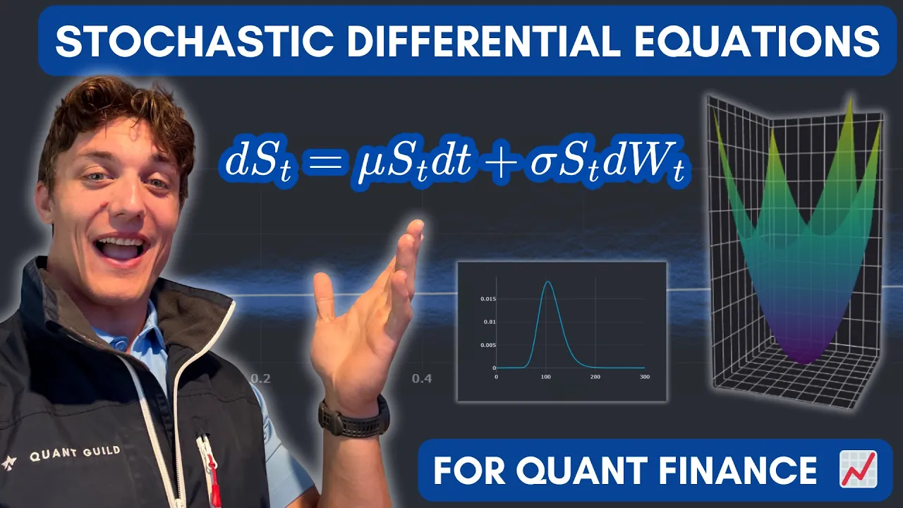
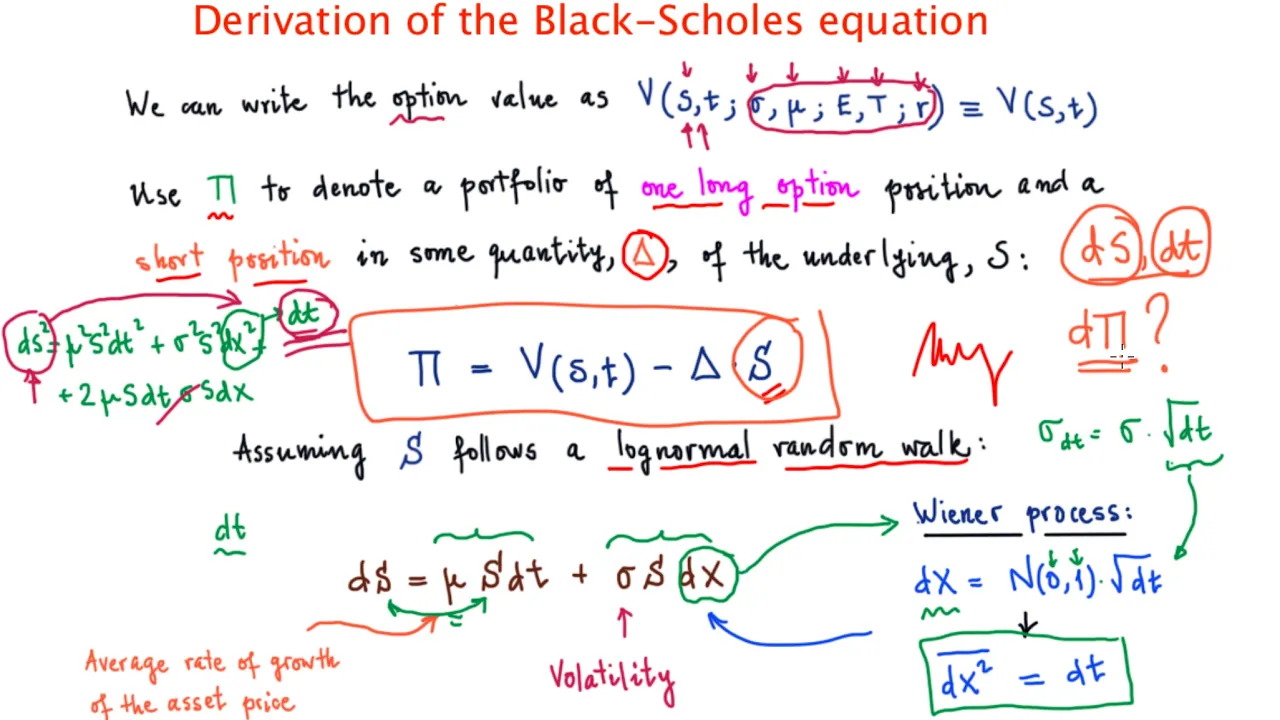










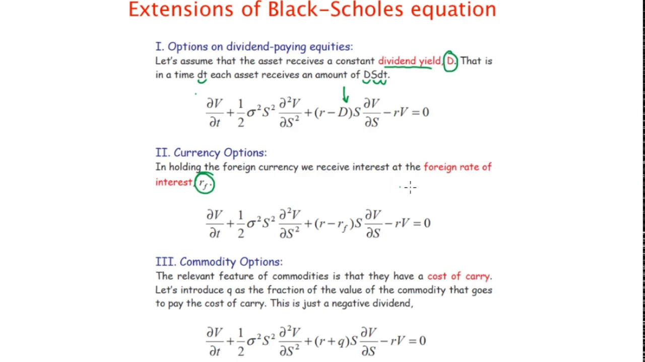


The Black-Scholes equation, derived using replicating portfolio arguments and stochastic calculus, provides an exact pricing formula for financial derivatives by assuming the underlying stock follows geometric Brownian motion; this equation shows that derivative prices depend only on volatility and risk-free rate (not expected return), and can be solved analytically for simple contracts like calls and puts, or numerically for more complex derivatives, with the key insight being that the value of any derivative equals the discounted expected payoff under risk-neutral probabilities.
Black-Scholes Equation: Mathematical Methods for Engineers
Added:Basic concepts of financial derivatives, particularly European call and put options, and the principle of no-arbitrage.
Introduction to stochastic calculus, including Brownian motion, geometric Brownian motion, and Itô's Lemma.
Fundamentals of partial differential equations (PDEs) and boundary value problems, as the Black-Scholes model is formulated as a PDE.
Standard probability theory, joint distributions, and the concept of expectation in financial modeling.
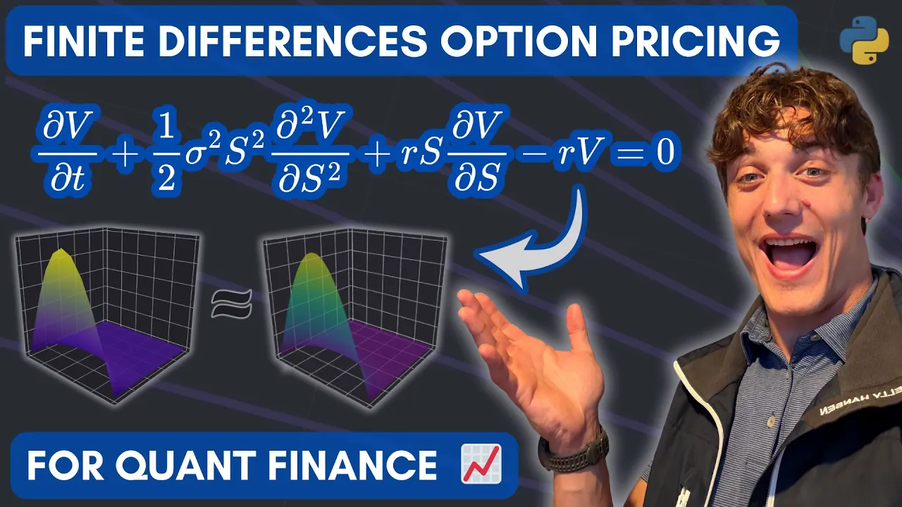
Implementation of numerical methods such as Finite Difference Methods (FDM) and Monte Carlo simulations to solve the Black-Scholes PDE.
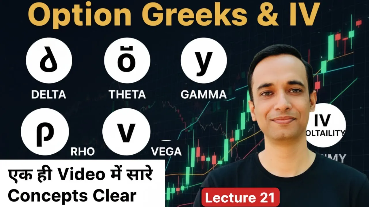
Understanding and calculating 'The Greeks' (Delta, Gamma, Vega, Theta, Rho) for portfolio risk management and dynamic hedging.
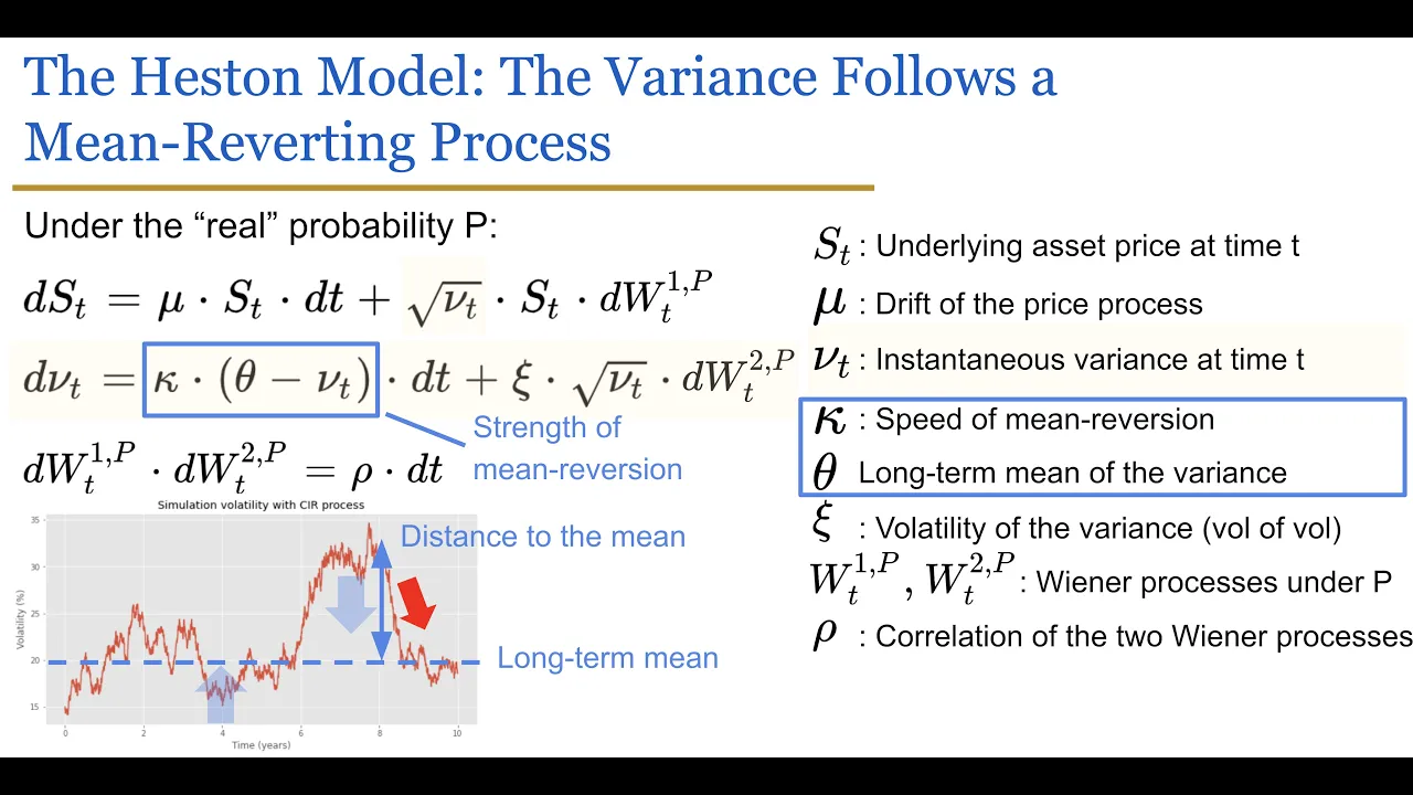
Exploration of advanced volatility models, including implied volatility surfaces and stochastic volatility models like the Heston Model.
Extension of the Black-Scholes framework to price exotic options and American-style options which lack simple closed-form solutions.
29.6K views46likes49:33Original Release: 2008-05-19
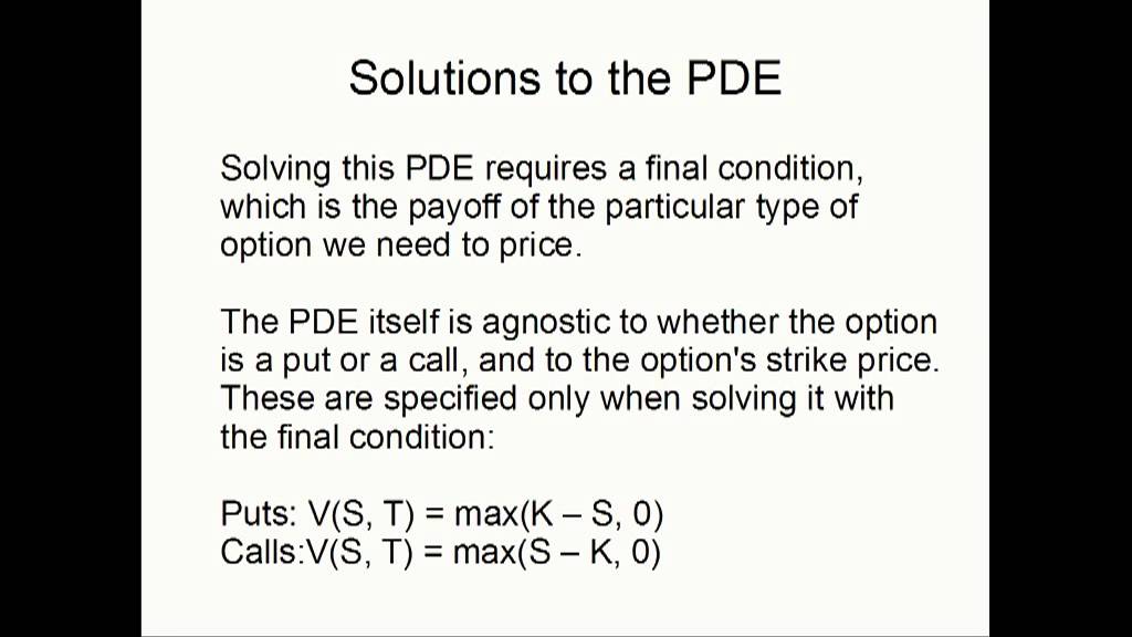
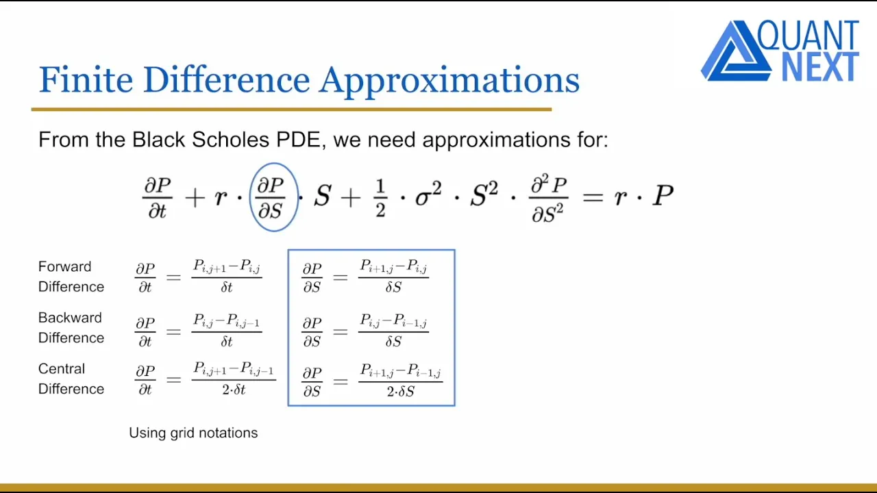
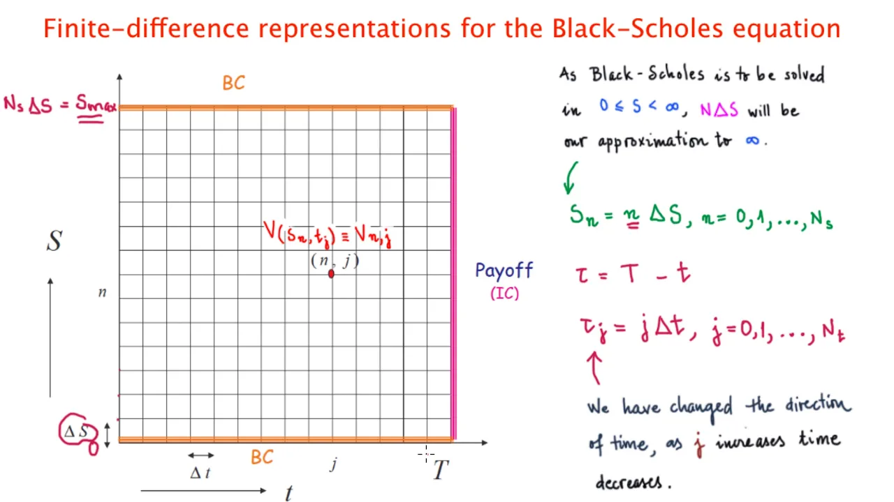
the following content is provided by MIT open courseware under a Creative Commons license additional information about our license and MIT open courseware in general is available at ocw.mit.edu vasia Vasa who uh works now for Morgan Stanley uh did his phc here in the mass department and kindly said he would tell us about uh Financial mathematics so uh so all your yeah so first of all uh let me thank Professor Strang for for giving this opportunity to talk here and it's it feels very good to be back be back to 1806 um so a few more words about myself I I've been Professor strank's student in mathematics uh about 10 years ago uh so after receiving my PhD i t me mathematics for a few years uh and then uh ended up uh working for a financial institution for a math Bank Morgan Stanley in particular uh and I'm part of uh analytic modeling group uh in fixed income Division and what we are doing uh we are doing Mass applications uh in finance and modeling uh derivatives fixed income derivatives and uh that's actually what I I'm going to talk about today I want to show how 1806 a Wonderful class which I admire a lot uh which applications it has in real world and in particular in finance and derivative pricing and let's start uh with a simple example which actually comes not from uh from Finance but rather from gambling uh well let's let's assume that well let's look at horse racing or cockroach racing if you prefer uh and Suppose there are two horses and sure enough people bet on them and bie uh is a clever one very scientific minded guy and he made a very good research of of previous history of these two horses um and he found out that the first horse has 20% chance to win and the second horse has 80% chance to win and he is actually right about his his uh his knowledge about chances to win on the other hand general public people who bat uh they don't have access to to all information and the bats are split slightly differently so there are the the the 10,000 is is placed on the first horse and 50,000 is placed on the second course uh Bui sticking to his uh scientific knowledge splits the odds 4 to one meaning that if the first horse wins then whoever put on the horse gets his money back and four times his money back on top of it or if the second horse wins then whoever put money on this horse will get the money back and one quarter of on on top of it so uh let's see uh what what are chances for uh for booki uh to win or or lose uh in this situation well if the first horse wins then he has to give back uh 10,000 plus 40,000 50,000 and he got 60,000 so he he gains 10,000 oh good good for him uh on the other hand if the second horse wins then he has to give back 50,000 plus a quarter of 50 which is 12 uh 12,500 so 6250 uh uh all together uh and he loses $2,500 and after many runs the expected win or loss of the bookmaker is the probability of the first horse to win times the expected win plus the probability of second horse to win times the expected loss which turns out to be exactly zero so in each particular run uh booki made may lose or win but he on uh on even he expects uh in the long run he he expect to break even on the other hand if he would put the chances he would set the odds according to the money bet 5 to one what would be the outcome well if the first horse wins he gives back 10,000 plus 50,000 6 60,000 exactly as he he uh exactly the the amount he collect Ed or if the second horse wins again he he gives back 50 plus 1/5 of that 60 he breaks even so no matter which horse wins in this scenario the Buie breaks even and how how Buie operat well he actually charges a fee for each B right so the second situation is much more preferable for him when when he doesn't care which which horse wins he just collects collects the fee while here he may lose or gain money and this is quite useful observation uh which uh which we will see how uh how it works uh in derivatives so now back to finance uh back to derivatives so we are actually interested in pricing a few Financial derivatives and what is a financial derivative well Financial derivative is a contract pay off of which at maturity at some time t depends uh on underlying uh underlying Security in our case it we always will be talking about a stock as underlying security uh and probably interest rates uh what are the examples of uh of of financial derivatives well the the most simple example is a is probably a forward contract forward contract is a contract when you agree to purchase the security for a price which is set today you agree to purchase the security in the future for the price agreed today well for example if you needed thousand barrel of uh of oil to heat your uh your house but not today but uh but rather for the next winter uh on the other hand you don't want to take the risks uh of of waiting until the next winter and and buying uh oil then you would rather agree on the price now and pay it uh paid in the future and get get the oil what the price should be what the price what is the fair price for this contract um uh well we'll see how to price it well uh the the the few observations here is that this this line represents the payout it's it's always useful to represent the payout graphically this is just a straight line because the payout of our contract is s minus k at time T and this actually gives the current price of the contract for all different bers of the underlying uh and usually uh the price of the forward contract is set such that for the current value of the underlying the price of the contract is zero so you it's it costs nothing to enter a forward contract so that's why it intersects zero here what are other uh common uh derivatives another common derivative is are calls and PS and I put European colon put here uh don't be confused by European or American it has nothing to do neither with Europe or or America it has to do uh of uh with the structure of the of the contract European B basically means that the the the contract expires at certain time T America means that you can exercise this contract at any time between now and and future we'll be we'll be talking only about European contracts so European call option is the contract which uh gives you the right but not obligation to purchase the underlying security at a set price K which is called stri strike price at a future time T which is expiration time so uh if your security at time T ends up below K below the strike then sure enough there is no point of buying uh of buying uh buying the security for for more expensive price so the the contract expires worthless on the other hand if your stock is ends up being greater than k at expiration time T then you would make money by by purchasing this stock 4K and your payout will be S minus K and this is a graph of your payout and this uh line here as we will see is the the current price of the contract and we'll see see how to obtain this line uh in a few minutes uh another common contract uh is is a put well while call was basically a bet that your stock will grow right uh the put is the B uh that that your stock will not grow so in this in this case uh the put is the right but not uh the obligation to sell the stock for for certain price K and here is the payout uh which is similar to the put but just flipped uh and this is the current price of of a put option call and puts being very common contracts uh are are traded uh on exchanges Chicago Exchange is uh is probably uh the most common uh place for the option for calls and puts on stocks to trade I just printed out a Bloomberg screen uh which uh which gives you information or about a few calls and puts on uh on IBM stock so I did it uh on March 8th uh and the IBM stock was trading at this time at 8114 and here are descriptions of the contract they expire on 2 22nd of April so it's pretty short dated contract uh they can go as far as two years from now usually and here here is a set of strikes and here are a set of prices and as as you can see there are there is no single price there is always a bid and ask and that's how dealers and Brokers make their money like like auki they they basically charge you a fee for for selling or or buying the the contract and U they uh and that's that's how the the money are made they are made on the spread but not on the price of the contract itself because as we'll see in a second we actually can't price the uh the the contract exactly and there is no uncertainty once the the price of the stock is Set uh there are plenty of other uh options slightly more exotic contract is a digital which pays either zero uh or one depending on where your your stock ends up uh it probably is not exchange traded Al I'm not sure uh there are there are hundreds if not sent of of exotic options where you can say that well how much would be the right to purchase this stock for the maximum price between today and uh two years from now so it will be past dependent depending on how the stock will go uh the payout will be defined by this path uh there are American options where where you can exet option anytime between now and maturity and so on and so forth so uh just before we go into mathematics of option pricing pricing uh just a few observations uh so uh and statements that first of all it turns out that thanks to to developed mathematics mathematical Theory uh if you make certain assumptions on the Dynamics of the stock then there is no uncertainty uh in in the price of the option you can say exactly how the option uh how much the option costs now and uh that's what uh provides that's and this is a big driver for the markets so so dealers quote uh these these contracts and there is a great agreement on the prices uh the price uh of the stock of of the uh of the derivative contract is defined completely by the stock price and not by risk preferences of the market participants uh so it doesn't matter what are your views on uh on the growth prospects of the stock uh the it will not affect uh the the price of of the derivative contract um and as I said so the the mathematical uh part of it comes into giving the exact price uh without any uncertainty so let's let's consider a simple example now let's assume that we are in a very simple World well first of all in our world there are only three objects the stock itself the riskless money market account meaning that uh it is an account where we can either borrow money or invest money at at a riskless rate R and uh finally our derivative contract here we we we are not making any assumptions on what kind of derivative contract uh it is it could be forward it could be call it could be put it can be anything moreover our world is so simple but first of all it's discrete and second of all there is only one time step to the expiration of our Contra DT and not only there is only one step left we actually know for sure we know exactly what are transition probabilities there are only two states at the end and we know the transition probability so with probability P we move from the state zero to the state one and with probability 1 minus P we move to the state two right and uh just notice because this is riskless money market account it it's the same in both in both cases right you you just invest money and it grows with with the risk-free inate so what can we say about the price of our derivative F Well it's simple minded uh well let's start with uh with with with the forward contract we know what the payout in delta T of our forward contract will be it will be just the difference between the stock price and and and and our strike well I simple mind that approach would be well we know the pro the transition probabilities let's just compute the expected value of our contract and that's what we would expect to get uh if if there were many such experiments well you take the probability of going to State one you multip by the payoff at State one you take minus P probability going to state two multiply by the the payout in in the state two you sum them up and you get this this expression and as as I said the common uh common thing to choose the strike such that the the contract is has zero value now so you get your strike well in particular you could say that if you research the market well and you know that the stock has equal probability of going up and down then actually your strike you you expect your strike to be uh an average of of two uh of two voles end voles of the stock but as we can imagine following our Booky example this is not the right price there is actually a definite price which doesn't depend on transition probability and here is the reason reason why there is a definite price well let's let's just consider a very simple strategy let's borrow just enough to purchase a stock so let's borrow s0 right now and buy the stock for the for this money and let's enter the forward contract well by definition forward contract has price zero now so we enter a forward contract now at time DT when our contract expires what happens well we deliver our stock which we already have in our hands for uh an exchange of K do that's our forward contract on the other hand we have to repay our loan and because it was a loan it grew it grew to s0 uh times e to e to the rdt now let's see what would happen if K was greater than S times to the rdt then we know for sure we know now for sure that uh that we we would make we we would make money there is no uncertainty about it now similarly if K is less than this value then we know that we will lose money and that's not how the r rational Market works if everybody knew that by by setting this price you would make money they people would do it all day long right and make infinite money and well so there will be no other side of of the market so the price has to go down so the only choice for K the only the only Market implied choice is that K has to be equal to e uh to S times e to the rdt right and as you can see it doesn't depend on transition probabilities at all that's what Market implies us and that's that's the price of forward contract and that's actually explains why when I was plotting the forward contract current price was just the the straight line it's just discounted discounted payoff there is it's the payout is linear so it's just to the parallel to to payout and uh so and that's the idea basically uh the idea is to try to find such a portfolio of stock and the money market account that with with such a payout which will exactly replicate the payout of of our derivative and if we found such a pfolio then we we know for sure that the value of this portfolio the replicating portfolio today is equal to the value of the derivative because otherwise you would make or lose money riskless that's uh that's no Arbitrage condition so uh can we apply it to our general One Step uh onestep World well so what we if we have a general payout F what we want to do we want to form a a replicating portfolio such that at expiration time it will replicate our payouts right so we want to choose such constant A and B that the combinate such that the combination of a stock and money market account in both States will replicate the pay the the payout of our option then if we if we are able to find such constants A and B then we just look at the current price of the of the contract and it has to be equal to the current price of of our deriv well but in our particular case this this is easy it's just two linear equations with two unknowns easily easily solved and here is current current price of our derivative no matter what payout is I mean you just substitute the payout here and you know if you know S1 s N2 and S2 that's it a useful way to look at it just to rewrite this equation is in this form and then notice that actually the price the current price of our derivative can be viewed as a discounted expected payout of the derivative but with very certain probability this probability is not it doesn't come from from statistical properties of the stock or or from any research it actually is defined by the market so it's called a risk neutral probability so uh this this probability doesn't doesn't depend uh on this uh on the uh views on the market by by the uh by the market participants and an interesting observation is that actually the value of the stock the discounted value of the stock is actually also is expected value of of the of our outcomes under this risk neutral probability and that's basically general idea now let's move one notch up and try to apply these idea to uh to continuous case well if we live in continuous world now we need to make some assumptions uh on on the Behavior Uh of of the stock right and a very common assumption is is uh that the the the Dynamics of the stock is log normal log normal meaning that the logarithm of the stock is actually normally distributed right so here U is some drift uh Sigma is the volatility of our stock and DW is a winner winner process uh W is a winner process such that DW is normally distributed with mean zero and Varan square root DT and our approach would be to find replicating portfolio and what does it mean it means that we want to find such constants over time DT so we assume that A and B are constant over over next step DT such that the change in our uh in our derivative is a linear combination with these constants of our underlying uh of the change of our underlying security and the change of money market account now uh now we just need to look more more closely at at at this equation and first of all let's concentrate on DF so F our our our our derivative is a function of stock value and time right but unfortunately our stock value is stochastic so DF is not that simple and to write DF out we we use uh we have to use a famous e formula from stochastic calculus which actually just tells you uh which actually is is analog of of of stor formula for stochastic variables well let's let's see if if our s will not be sastic if it would be completely deterministic and depend only on DT then there would be no term and differential of f is just a standard standard expression on the other hand if uh if we have dependence uh on on on stochastic variables then we have we have to have more terms and why this happens well in very rough words is that because the order of magnitude of thew is higher than than DT it's it's square root of DT right so we have we have to make into account more terms and uh in particular we have to to to take into account next next order of DS squ and formally DS squ can be written this way and again very rough explanation is as follows if we if would square if would Square this equation there will be three terms there one would come from the square of this term and which order this would be it would be of of the order of DT squared next order of magnitude right much smaller than DT second term will be cross product of DW DT what kind of what what order of magnitude we are talking about it is DT to to the^ three Hales again against much smaller than than DT on the other hand the third term will be the square of DW which is of order of magnitude of DT so that's what we have to keep right and that's what either formula is is about okay now uh now we we are basically we know all terms here and let me uh stress out that this term DB it is not stochastic it's it's completely deterministic and uh because we know that b grows with the rate R that's that's what it is so we substitute all those terms into our replicating equation we collect the terms we get this equation and again there is deterministic part there is stochastic part so the only way for this equation to hold is uh this term to be equal to this term and this equal this term to be equal to this term and that's what's written out here so again two equations these two unknowns and here is the answer finally let's look let's take a s to to another part and notice that this part of our equation is completely deterministic right so we know how it will grow so basically D of f minus a s which is d b b * DB is R * B * DT and we know all other terms we substitute them here take something to the left left hand side and get this equation so this is partial differential equation uh for uh for our our derivative f as a function of s and t of second order um and this uh this equation is a famous black schz equation which was derived by Fisher black and mil mil schz in their famous paper published in 1973 and Marin sches and Robert Martin actually received Nobel Prize for for for deriving and solving this equation in 97 uh black was already dead by that time uh so and this is really the Cornerstone of of of mass Finance the the and the Cornerstone is because using the the replicating portfolio using uh the this reasoning we were able to to find a an exact equation for our derivative so a few remarks on black schs so first of all we wa we made some uh some assumptions on the dynamic of the stock but we've never made any assumptions on on on our derivative which means that any derivative has to satisfy this equation and that's very very strong result so if you assume that our stock is log normal which is not a bad assumption uh and agrees quite well with the market then we basically in principle can price any derivative we know the equation for for any derivative the other thing is that our black shs equation doesn't depend on the actual drift mu of of our in the Dynamics of our stock so again it is it is the uh the Manifest of risk neutral uh risk neutral Dynamic not only we uh we wrote down the equation for for our derivative we also found a replicating portfolio so in other words we found a heding strategy meaning that at any given time we can form this portfolio with weights A and B and if we hold both the derivative and both the replicating portfolio all together the the the this is zero sum gain we know that no matter where stock moves we will not lose money or gain money so if if we just charge bid offer on on on the derivative we if we charge a fee on the contract we can hedge ourself perfectly buy the contract and or sell the contract hedge perfectly cly ourselves and just make money on the fee that's it um and finally more mathematical remark is that actually after a few manipulation a few change of variables the black shs equation comes out to be just a heat equation which which you already saw in this class and and this is very good news why this is good news well because he equation is very well studied so so the solutions are are well known and numerical methods the ways to solve it in particular the numerical ways to solve it are are well known so we are in business but as any partial differential equation uh the the equation itself uh doesn't make much sense because to find a particular solution we need boundary uh and an initial an initial condition and if uh if and although any any derivative satisfies black schs equation the the final and boundary conditions must uh will vary uh from contract to contract and here are a few examples of the final and boundary conditions and here the an interesting remark that if usually we would talk about initial conditions here we we are talking about uh final condition the time goes in reverse we know the state of the world at the end at expiration not not today so um the here are final and Boundary condition for colon putut and let's look a little bit at the pictures for our Co put to see where they come from so for example for Co well this is our final condition right which is defined by by the payout on the other boundary conditions well what happens we we put them at zero at at an Infinity we show that to put them at zero at infinity and why well because if stock hits zero then it stays at zero that's that's what what our Dynamics shows so the value of our contract at at maturity will be will be just zero on the other hand if the stock grows uh grows to Infinity a good assumption to make is that actually it becomes similar to stock itself so it just becomes parallel to the stock and that's uh that's the uh the conditions which we impose here no similar for the put uh you can derve these conditions and again just because it is a heat equation it turns out that for for simple derivative such that that calls in puts it is possible to find an exact analytic solution and here here are exact analytic solutions for call put and the digital contract uh well not not surprising again I mean they they are all connected to to to the error function so to the normal distribution basically as as the the solutions of heat equation ought to be um why do they look exactly the same if we have uh five minutes at the end we we will probably shed some light on on the specific form of of equations but let me just stress that we can see that it's it's discounted and what I'm claiming it's expected value of of our payout under risk neutral measure and here here is an example of a particular uh particular call option on the same IBM stock uh so I chose a short dated contract just to avoid uh the the the dividend payments so it's a contract expiring on March 18th so there there is 10 days to expiration uh the dra the stock as as we saw uh so this exploration the stock as we saw is was trading at at h14 the volatility is somewhere around 14% uh they estimated either from from other options or from or historically and here is the price of our contract and I also have a simple black shs calculator here and let's see if we can match this price so let's see uh what was it was I believe the volatility was 133% right 1347 uh the interest rate or it's already here as as we all know fed just bumped the interest rate so they are at 4.75% right now uh the the strike of of our option uh was 80 time to expiration was actually 10 days and this should be measured as a fraction of year so we divide 10 by 365 uh and the stock was trading at 8114 if if I'm not mistaken and here is the price of our co-option contract which is 150 well well it's it's within within with offer right so maybe our volatility slightly off and if you increase increase it to say oh uh increase it to 14% it will go slightly slightly up yeah 5502 well in general let's play a little bit uh with it so just well it is very short dated option so the uh the value of our option is very close to to to the payout so if we increase the time to to maturity let's make it two years just to see better so now now value of our option is well that's that's what what it is and if we increase volatility sure enough let's make it 30% so what do we expect we expect if volatility is higher then certainty is higher so the value of our contract should go up and it sure does right uh yeah so so basically that's how black shs works and plenty of those contracts trade on the market but unfortunately not all of these contracts are so simple as calls and puts well first of all there are there are many more complicated uh complicated products with uh uh more difficult uh payouts which will constitute different and probably discontinuous uh final conditions on on our black sh equation uh moreover uh we made an assumption that the volatility is constant with time and interest rate is constant with time which is certainly is not true for the real world uh volatility probably should be time dependent and this would make the coefficients in our black shs equation time dependent and unfortunately this cannot be solved analytically so in most of the cases in practice we will have to use some kind of of numerical solution and uh finding difference methods uh is a typical approach for for the heat equation as you know both explicit and implicit uh schemes and uh you you will discuss some in some of those in in in 1886 three methods three methods meaning that uh we go back to our one step three and basically assume that our our time to expiration is many time steps away and we'll grow this tree further so from this node we have two more nodes and so on and so forth then you would imply the uh the final condition at the end and discount back using our risk neutral probabilities and get the price now so those are called three methods and one can show that actually those three methods are equivalent to uh to fin a uh difference explicit find a difference schemes those are very popular uh but again in in three methods what what is very important is to set the probabilities on your Tre the transition probabilities to the right ones and the right ones are risk neutral probabilities probabilities implied by the market actually um another uh important numerical method is is Monte Carlo simulation where you would you would simulate many different scenarios of the development of your stock after the maturity and then basically find uh uh using this path you you you will find the uh the expected uh value of of your of your payout but again in order for this expected value to be the same as as as the risk neutral value as as the Arbitrage free value you have to to develop your multicar simulation with risk neutral probabilities so risk neutral valuation is is extremely important uh and here is actually the general risk neutral statement which one can prove is that actually the value of any derivative is just discounted expected value of the payout of this derivative at much mat but you have to to take this expectation at the right measure using the right measure meaning that you have to set correctly the transition probabilities you have to make them Mark uh uh Market neutral uh and under this measure actually the uh the the Dynamics uh of of the uh of our stocks looks slightly different and as you can see our drift becomes the interest rate so under risk neutral measure Everything grows with with our risk-free interest rate and just to shed a little bit of light on what on how um we we got the solutions uh for for calls and puts black solutions for col and put well this is the distribution of our stock log normal distribution of our stock at time T and if we take this distribution and integrate our payout of our call option against this distribution in other words in other words find uh find the uh the expected value of of payout of our call option under risk neutral measure then sure enough sure enough you will get to this formulas and this illustrates the best because what is digital digital is just the probability to end up above the strike at time T right so if you integrate this log normal PDF from uh from the strike K to the infinity that's that that will be your your answer and this is a good exercise in integration to make sure that it's correct so let's see to conclude what we we have seen so uh so we have seen that modern derivatives business makes use of of quite advanced mathematics and what kinds of uh of mathematics is used there well partial differential equations are used heavily numerical methods for the solution of these partial uh differential equations are naturally used in order to get this these equations we we we actually need to to operate in terms of tastic calculus meaning that we we need to know how to deal with EA calculus EA formula Gano theorem and and so on and so forth the other thing is uh is to be able to build simulations uh to solve the the heat equation and uh and all other equations which you might might encounter the the topic which we didn't uh didn't touch upon is statistics because of course Very Advanced statistics is used for for many uh many things for analyzing historical data uh which is can be quite useful for trading strategies and uh and many others and besides these five topics there is much much more to uh to mathematical Finance uh which which make it a very very exciting field uh to work in and that's what uh I wanted to talk about and thank you very much for your attention so maybe I'll ask ask a first question about boundary conditions right because you said that those are different for different uh contracts and uh how do you deal with them in the finite differences or the tree model or whatever well so uh what would be a typical one well typical one yeah here are two very typical ones yeah so uh those you set them uh you you basically make a grid of your uh of your problem of your uh in particular you you build a tree right which is actually a grid of all possible outcomes uh you set them up at the end so your threee grows so you set your boundary here at the at the end and uh well you you set probably uh some initial uh and um well this is final condition so you set some boundary conditions here right so this is your time T this is t0 this time T this is zero this is one this is two this is T right so you set your payout here so it will be maximum of of S minus K n0 right so how many time steps might you take in a well well you would do like day daily for three months if it's three months option something maybe 100 yeah something like that well if it's two two two year option that you probably would do it weekly or something like that so you don't get into large what would be scientifically large scale no no no in finance you usually don't get don't hit this problem of and in finite differences do you use like higher order that suppose you had second derivatives do would you always use second differences or I mean second order accuracy or in in general yes in general second order accuracy yes you you in general you don't you don't go higher yeah I mean they the Precision well it's within sents right yeah so you you can do better than that so so it depends uh well it depends what kind of amounts you're dealing with if if you actually selling and and buying billions of stock you might consider something I see something more precise but but it's it's it's very def it's very problem to find so so yeah that's how we deal with that any questions you can put the mic on if you have a question this is a little can you solve it actually formulating the problem as a mark of process Mark of change we must have this structure right well it it is Mark of process it yeah I mean this is just a numerical solution so yeah it is Mark of process and basically all stochastic calculus is about Mark of process continuous Mark of process yeah true enough and is the mathematics that you get involved with pretty well set now or is there is there a need for more um more mathematics if I can ask the question that way yeah well uh in this field it is probably quite well set yeah but if you get into more complicated fields and especially into credit modeling uh the the model for uh for the credits of certain companies then mathematics is not quite set because there you you start talking about jump processes and not winner processes not not just L normal processes and this partial different I mean stochastic differential equation become very hard but maybe still analytically tractable so uh from this point of view there there is need but it's uh it's not a fundamental mathematics not that you're opening a new field but definitely trying to solve a stochastic differential equation which usually boils down to solving a partial differential equation right analytically uhhuh can be pretty hard in mathematical problem purely mathematical problem and and you so you showed us the example of a St black skulls solver right uh do everybody has that available all the time oh yeah on on CH Chicago trading floor the the Traders have calculators where they just press a button and it it's just hardwire there and they're printing out error functions basic combination of error functions yeah that's all it well sure enough nobody uses just I mean this was very approximate example and that's why I chose such short dated stock that before it pays any dividend and where we can assume that the volatility is constant and so on and so forth to match the prices otherwise the uh the price will match thank you thank you
Up Next
5:54
Physical Chemistry Math Review: Foundational Topics and Skills
@TMPChem
26.8K views•2017-03-16

4:43
Elliptic Curve Cryptography Explained: ECC, ECDSA, ECDH
@PracticalNetworking
28.5K views•2024-10-21

20:22
Cantor's Theorem: Proof & Diagonal Argument | MIT 6.042J
@mitocw
33.1K views•2016-09-12

6:00
The Mathematical Impossibility of Accurate World Maps
@Vox
23.3M views•2016-12-02
Related Study Plans & Knowledge Roadmaps
Structured learning paths in Mathematics
mathematics
Tensor Calculus: Vectors to Riemann Curvature
01Mathematical Foundations: Linear Algebra & Calculus
02Covectors, Dual Spaces, and Tensor Basics
03The Metric Tensor and Index Gymnastics
+ 2 more learning modules
40h5 modules
Explore Roadmap
mathematics
Gödel's Incompleteness: Logic, Proofs & Limits
01Introduction to Formal Systems & Hilbert's Dream
02Set Theory, Cardinality, and Cantor's Diagonal Argument
03Arithmetization and Gödel Numbering
+ 2 more learning modules
14h5 modules
Explore Roadmap
mathematics
Galois Theory: Fields, Groups & Solvability
01Foundations of Abstract Algebra: Groups & Fields
02Polynomials & Field Extensions
03Splitting Fields & Symmetries
+ 2 more learning modules
24h5 modules
Explore Roadmap
mathematics
Non-Euclidean Geometry: Models & Geodesics
01Euclid's Fifth Postulate and the Birth of New Geometries
02Hyperbolic Space and the Poincaré Disk Model
03Geodesics: Defining Straight Lines in Curved Spaces
+ 2 more learning modules
15h5 modules
Explore Roadmap