




![Data Science Lecture 5: Support vector machines [part of the IDS course @RWTH]](https://i.ytimg.com/vi_webp/v_hJF8v4UKc/maxresdefault.webp)



![Zustandsraumdarstellung #1 [Technische Mechanik] |StudyHelp](https://i.ytimg.com/vi_webp/GcQEbZrRriM/maxresdefault.webp)

![[Fondamenti Controlli Automatici] - Lez. 02](https://i.ytimg.com/vi/PJ1I3b2RMvA/hqdefault.jpg)










![732 - Showcasing SimStructure (TempleOS) [2016]](https://i.ytimg.com/vi/zIEAxPgV5QQ/maxresdefault.jpg)
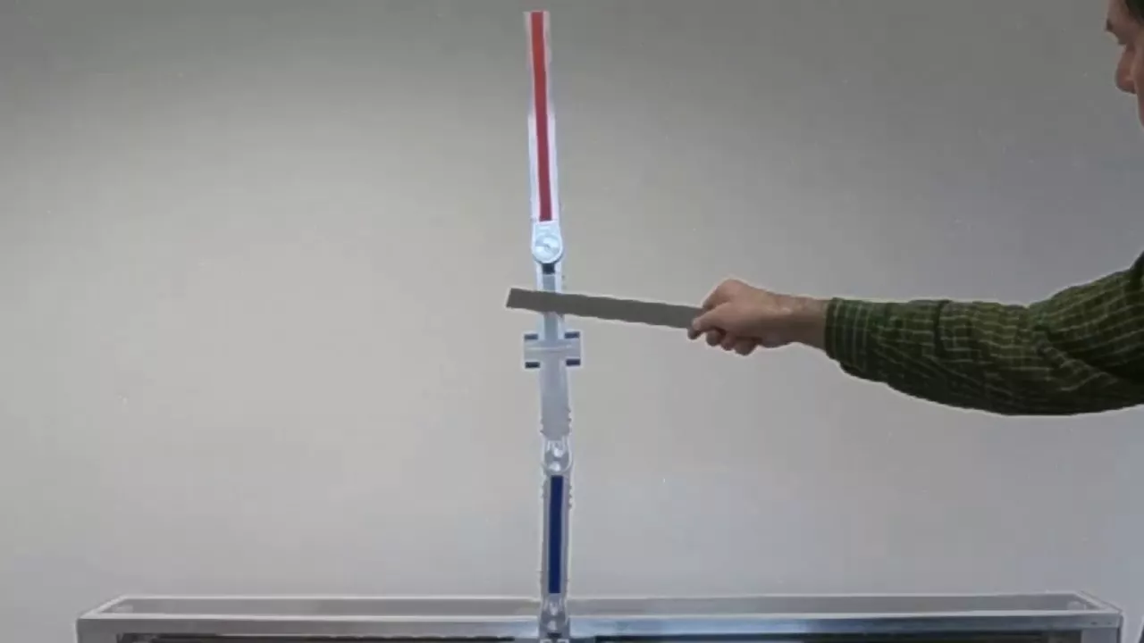


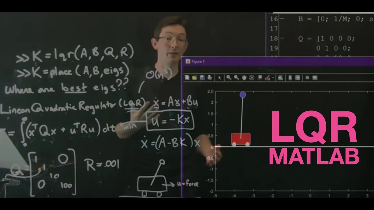
The inverted pendulum on a cart system demonstrates that a two-degree-of-freedom nonlinear system with state variables (cart position, cart velocity, pendulum angle, pendulum angular velocity) can be analyzed for controllability by linearizing about fixed points (pendulum down at θ=0 and pendulum up at θ=π), computing the Jacobian to obtain the A and B matrices, and verifying that the controllability matrix has full rank (rank=4 for this system), which confirms that the system is controllable and allows for eigenvalue placement through state feedback control.
Inverted Pendulum on a Cart: State-Space & Control
Added:Foundational Classical Dynamics: Understanding how to derive equations of motion using Newtonian or Lagrangian mechanics for multi-body systems.
Linear Algebra Essentials: Familiarity with matrix operations, eigenvalues, eigenvectors, and system of linear equations.
Introduction to State-Space Representation: Basic understanding of representing dynamical systems using state vectors and state-space equations (A, B, C, D matrices).
Linearization of Nonlinear Systems: Understanding how to linearize nonlinear differential equations around an equilibrium point using Taylor series expansion.
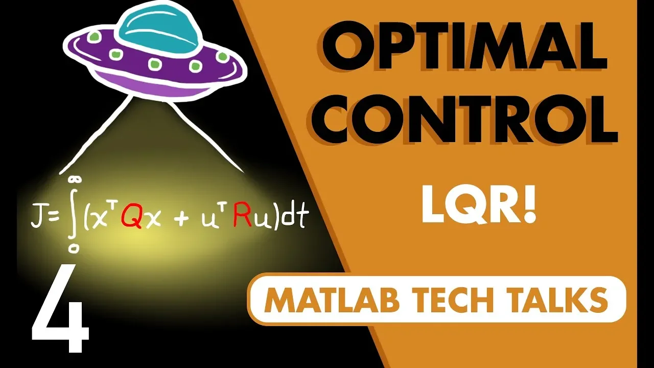
Optimal Control Design (LQR): Learning how to design a Linear Quadratic Regulator to stabilize the inverted pendulum efficiently.
State Estimation and Observer Design: Implementing Kalman Filters or Luenberger Observers to estimate unmeasured states, such as pendulum angular velocity.
Nonlinear and Robust Control: Exploring advanced control strategies like Sliding Mode Control or H-infinity control to handle parameter uncertainties and larger angle deviations.
Trajectory Tracking and Swing-up Control: Designing algorithms that can automatically swing the pendulum up from the hanging position before stabilizing it at the upright position.
278.5K views3.8Klikes15:08Original Release: 2017-01-29
welcome back so now we're actually going to start coding up real examples in mat lab seeing if they're controllable designing controllers uh to stabilize the dynamic so this should be really fun and really powerful okay we did a lot of math to understand why and when and how to control things but now the rubber is going to hit the road and we're actually going to see how easy it is to really control a system in mat lab okay so one of the systems I really like to to work with is imagine that I have um an inverted pendulum but that inverted pendulum is sitting on top of a cart okay and so I'm going to have my inverted pendulum but now that pendulum is on a cart and I can move that cart around so for some reason this is always felt much more physical to me than just you know having a pendulum with some torque control on the bottom that seems too easy this is a little more interesting right I have some cart and I can move that cart around and I'm trying to stabilize this inverted pendulum okay so let's think about what numbers we need um well first of all we need to define the state of the system okay and so the state of the system is given by uh the position of this cart we're going to call that X and the uh angle of this pendulum arm we're going to call that Theta so so our kind of high dimensional dynamical System state um I'm going to change it up and I'm going to call it a vector y so this state y dot yeah maybe I'm not going to call it y because that'll be confusing with the output measurements let's keep it X the vector of States I'm going to say is this position script X its velocity script x dot Theta and Theta dot okay and so this is a twod degree of Freedom system there's two degrees of freedom X and Theta the position of the cart and the angle of the pendulum and because it's two degrees of freedom with Newton's 2 law I get four coupled Odes okay so I essentially have some uh DDT of x equals some nonlinear function of that Vector X so this is four nonlinear row equations I'm not going to bore you with the details of how to actually derive these but you could use something like Oiler lrange equations or Hamilton's equations and you could get these coupled first order nonlinear Odes okay so this is an honest to goodness nonlinear problem but we can linearize the system and just intuitively we know that there are a couple of key fixed points okay so the fixed point point of the system fixed points we're going to have um a fixed Point corresponding to the pendulum down position so what we know has to happen is Theta has to equal either zero for the pendulum down or Pi for the pendulum up um Theta dot has to equal zero x dot has to equal zero and if I wrote down all of these equations you'd see that none of these uh rates of change actually depend on X itself and so X is a free variable and that kind of makes sense right it doesn't matter if this thing is here or here or here if I have the the pendulum up or down and there's no velocities it's a fixed point so I've got two basic fixed points corresponding to let's say the Theta equals z case is the pendulum down with the Cart fixed and the theta equals Pi is going to be the pendulum up with the Cart fixed okay and so if you had the oiler lrange equations and you had these fixed points you could compute the Jacobian and you could essentially get um you know so through DF DX evaluated at a fixed point you could get uh a linear system of equations X do equals ax + b u okay and now I haven't told you what what U is this is super important so you the control input for this system what we're going to get to control we're going to say that that U equals a force on the cart in the X Direction okay and this is actually very reasonable what I can do is I could have like a motor on one of these wheels and I could have some controller so that I could if I specified I want you know twice the force I could give it twice the voltage and make this thing move okay so this is actually very realistic you could build a cart that would hold this pendulum and drive it around and you could actuate with Force okay and so now what I'm going to do is I'm just going to fire up mat lab and show you I've already cooked up all of these examples so I have this nice function so in mat lab right I build these right- hand side functions this is my nonlinear OD it's called cart pend the cart pendulum system and it gives me uh the time derivative given the state so here it's called y That's why I wanted to call it y sometimes in mat lab you call these states y That's just kind of mat lab convention and a couple of other numbers I just have a bunch of parameters out here so I say that this little Mass has mass Little M the cart has mass Big M uh this inverted pendulum has a length L uh we know that gravity pulls down and then there's D which is essential some damping term okay so in these equations there could be some friction um I believe I mean the damping to be as opposing the x dot okay so it's a damping on the cart maybe this cart has some friction and I'm assuming the pendulum has a lot less friction and then finally I have this U so if I was going to apply a force you can derive Oiler lrange or Hamilton's with some Force applied and I'm not going to bore you with all the details there's going to be a link to this uh on YouTube so you can download this code and read through it yourself but the right hand side these Dynamics are pretty nasty okay this actually takes a long time to derive by hand on pencil and paper for the system this is the most timec consuming part of this whole demo is actually getting this right- hand side Vector uh Vector field right but I'm not going to bore you with the details um you can see like if I go on and on it's a pretty long nasty expression okay um and the input the force enters in the x dot and the Theta dot equations when you go through oilo lrange that's what you find okay no big deal um it's just a nonlinear right hand side and this is relatively easy to simulate the system with or without forcing in Matlab so I'm going to go up to this function called Sim cart pend and all I do is I specify some parameters so I say this is mass one this is mass 5 length is two gravity is normal and there's some moderate dissipation on the cart and in mat lab I can integrate Vector Fields using OD 45 so I can integrate this if I set up some time span so I I want to integrate from 0 to time 10 with this initial condition so and again this initial condition means X is Zer x dot is zero Theta is pi so it's up and Theta dot is 05 so it starts in the up position but it's moving in the to the right I think or you know in the positive Theta Direction maybe it's to the left but anyway then I go through and I write this o45 I tell it that I want to integrate uh X Y dot equals this function of Y and I'm going to lock in these parameters and there's zero control so for right now we're just going to simulate this thing in free physics with no forcing okay and down here at at the bottom I have a function I've written called Draw cart penned um and so essentially it just plots a movie of the pendulum and again you can download this and see what I did so let's actually try to run this Sim cart pended okay let's hope this runs and you can see this is basically what you expect to happen you let this thing go and it's going to just swing and swing and swing and eventually if I integrated it for longer it would come to rest maybe I'll just show you that cuz it's pretty easy I'll integrate it for a little bit longer okay it's going to go and it's just going to keep swinging and swinging and swinging and eventually friction will kick in and it'll kind of come to rest okay uh and it's only stuck here because I stopped integrating so that's the system we're going to control okay we're in a great shape to actually control this system so what we're going to do we know the fixed points I you know offline I computed this Jacobian matrix it was ugly and kind of a mess and I plugged in these fixed points so I have linearized equations about the pendulum up condition and I have linearized conditions about the pendulum down condition and so what we're going to do is we're going to simulate uh we're going to design controllers based on those linearizations and then apply them to the full honest to goodness nonlinear system okay so the first thing we need to do is get this Jacobian then we plug in the fixed points and either the pendulum up or pendulum down condition to get this linear system and then the first thing we need to do is check and see is this controllable okay so that's what we're going to do now I have this code here um called pole place cart pended okay um and what I've done here is offline I've essentially cooked up the a matrix and the B Matrix for this linearized system of equations and because the up linearization and the down linearization share so much in common I decided to have this little switch where if the pendulum is up the switch is one and if the pendulum is down the switch is negative one and so essentially this is the linearized Matrix the a matrix um for both conditions and if I want to go from pendulum up to pendulum down I just switch this s this s and this s to negative values okay so this is the a matrix and the B Matrix now all I want to do at this point is first of all I'm going to run this code so I'm going to run my I'm going to run pole place cart pend so it's going to load the a matrix and the B Matrix oh I think that ran the whole thing um so I'm going to load my a matrix and I'm going to look at I of a so these are the igen values of my a matrix in the pendulum up condition and notice that one of these I values is unstable so that thing is eventually if it's if it's Epsilon off of vertical it's going to um accelerate away now what's really important is I want to know what is a and b controllable okay so this was something we've been working up for up towards and it should be really easy to test now so I'm going to try first of all ctrb of a comma B this will give me that controllability matrix it's a big Matrix I'm just going to hit enter you'll see um right it's a big matrix it's a 4x4 Matrix so if I look at the the rank of this ctrb Matrix if this rank is four my system's controllable if this rank is not four the system is not controllable okay so with this a matrix and this B Matrix corresponding to force in the X direction of the cart because the rank of my controllability Matrix is four I can span all of my state space with this controllability Subspace and that means that I can actually develop a controller to control the system so what's coming next this will be in the next video we know it's controllable and so what that means is that I can cook up some control law U = minus KX so that the closed loop system is x dot equal a minus b k x and I can develop I can uh design K so that the igen values of this are anywhere I want them to be so what I'm going to do next is I'm going to specify I want stable IG values I want to move these igen values into the stable the stable left half plane so we had that one unstable IG value I'm going to move it into the stable left half plane with some proportional feedback of X and just to remember what this diagram looks like we have our system in this case the cart pendulum we're going to measure the full State X we're going to feed it back so U is going to be minus KX okay so we're literally going to say U equals minus this Matrix K times the measurements of X we're going to measure everything and that's going to stabilize the system to have these igen values so that's what we're going to do next we're going to use the place command in mat lab to place these igen values and Design This Matrix k then we're going to develop an optimal igen value placement using the linear quadratic regulator or lqr control so that's coming up next
Up Next

6:29
MPU6050 Gyro Calibration Guide: Raspberry Pi Pico W MicroPython
@mmshilleh
16.8K views•2022-12-17

30:32
Ultrasonic Transducers: Resonant Frequency Measurement and Horn Design
@imajeenyus42
229.9K views•2017-02-22
13:03
LQR Control for the Inverted Pendulum on a Cart: Full-State Design
@Eigensteve
243.5K views•2017-01-29

33:39
How a Student's Question Saved a NYC Skyscraper from Collapse
@veritasium
22.8M views•2025-04-26
Related Study Plans & Knowledge Roadmaps
Structured learning paths in Engineering
engineering
Building Acoustic Levitators: Physics & Arduino
01The Physics of Sound and Standing Waves
02Piezoelectric Transducers and H-Bridge Drivers
03Arduino Programming: Generating 40 kHz Signals
+ 2 more learning modules
14h5 modules
Explore Roadmap
engineering
Building Peltier Cloud Chambers: Particle Tracks
01Cosmic Rays & Cloud Chamber Physics
02Thermoelectric Cooling (TEC) Fundamentals
03Custom Liquid-Cooling Loop Design
+ 2 more learning modules
18h5 modules
Explore Roadmap
engineering
Yagi-Uda Antennas: Modeling, Build & VNA Test
01Introduction to RF and Antenna Fundamentals
02Yagi-Uda Antenna Design Principles
03Antenna Modeling and Simulation in 4NEC2
+ 2 more learning modules
18h5 modules
Explore Roadmap
engineering
ECG Monitor Design: Op-Amps, Filters & Noise
01Electronics & Breadboard Basics
02Op-Amps and Instrumentation Amplifiers
03Bioelectricity and ECG Fundamentals
+ 2 more learning modules
18h5 modules
Explore Roadmap