Public Economics and Finance: Intro to Public Finance

[00:00:10]Okay, so let's start off with what is public finance? Well, public finance is what I call it because it's what I was raised to call it, but it's also, you know, what it really is is public economics because what we're not going to be really talking about is the actual financing of government, right? We won't be talking about mun bonds and stuff like that. We'll be talking about deficits and debt. Come on in. um we'll be talking about deficits and debt and stuff like that to some degree to an entire lecture. In fact, we'll talk about government budgets. But we're not going to be talking about the MUN bond market. That's not going to happen. So really when I call it public finance, I mean public economics. Public economics is the study of the interaction or the role of government in the economy.

[00:00:44]Public finance seeks to answer three main questions. The first is when is there a role for government? When should government intervene in the economy? The second question is how might the government choose to intervene? What are the different ways in which it could intervene in the economy? It's different policy tools. And the final question is of these alternative alternative interventions, what are the potential effects of these different tools? So what are the direct effects? What are the indirect effects of these particular ways the government could intervene? So let's tackle the first question. When should the government intervene? Well, there's two main reasons the government might choose to intervene. The first being that there's some sense that there is a potential for redistribution that would be more optimal that somehow whatever the equilibrium in the economy is whatever the competitive equilibrium is is not achieving an allocation of resources that the society is pleased with.

[00:01:39]Society would like things divided up differently. In that case the competitive equilibrium won't handle that on its own. There are some special cases in which sort of the second fundamental theorem of welfare tells us that uh you know if we reallocate initial sort of resources the competitive equilibrium can then achieve any um postequilibrium allocation of resources but that takes the frictionless transfer of assets between people and that's generally pretty hard to do right it's very hard to just say hey Mr. Buffett, that's a fine billion dollars you have over there. We're just going to give it to Matt. You know, that's very it's not something society we typically are able to do. We call those transfers lumpsum taxes. And while they're a theoretical possibility, they're in actuality pretty hard to actually achieve. So in general, if we want the outcome, the equilibrium allocation of resources to be different, we need have we need to have something larger than the competitive competitive forces sort of intervening to redistribute resources. The second reason we might see a role for government, why government may have a role a role to play or a potential to improve the equilibrium is in the case of market failures. Market failures just mean that the competitive equilibrium isn't achieving sort of maximum efficiency that there are sort of missing blind spots in in the competitive equilibrium that uh government could potentially uh fix.

[00:02:55]What types of market failures am I talking about? The first is simply externalities. So the spillover of one person's uh uh so it's this case where one person's decisions spill over onto other people, right? Or other actors in the economy. There's a case of positive externalities like vaccinations, right?

[00:03:13]When I choose to get vaccinated against measles, I actually make other people better off, right? People who have no real people who aren't vaccinated are less likely to get measles if I'm unlikely to get it because I'm vaccinated. That's a positive externality. It might be true that when I'm well educated, I work better with other people. I'm less act I'm less sort of uh likely to commit crimes, etc., etc. That all benefits my community members, right? Because I'm less likely to inflict crime on them or I'm a more pleasant person to be around. So, that could be a positive externality of education. But there also negative externalities, right? The classic example being a paper mill that's upstream from say a fishing village. as the paper mill decides to perhaps dump, you know, say dioxin or something into the stream because that's the most cost-effective way for it to dispose of the dioxin, right? It's making a decision based on its profit function, its objective. But what does that have?

[00:04:04]A spillover. It has a spillover onto the onto the fisherman downstream because their productivity falls. For every hour they spend fishing, they catch fewer healthy fish, right? Because the water's polluted. That's a negative externality that the paper mill is exerting on the fisherman. Uh second, there's the there's a market failure if there are public goods. A public good is simply a good that is non-rival and non-excludable. Non-rival means the fact that I'm using it does not mean you can't use it. We can use it simultaneously. Non-excludable means I can't stop you from using it. The quintessential example of a public good is defense like national defense. If I contribute part of my tax dollars, say part of my tax dollars are going to build an aircraft carrier or let's say a missile missile defense system, I feel safer, right, because of the missile defense system. I can't prevent you from feeling safer, right? Once this missile defense system is in place and I can't uh been just because I'm feeling safer doesn't mean you can feel you can't feel safer. So defense is like the quintessential example of public goods.

[00:05:05]But there are other things too, right?

[00:05:07]Uh public goods could be uh caring for the homeless, right? If I spend $20 to distribute money towards the homeless, you may feel good that no one is on the streets, right? That's a public good.

[00:05:20]And I can't stop you from feeling that way. And because I feel good that no one is on the streets doesn't mean you can't feel good that no one is on the streets.

[00:05:26]So these are many types of public goods.

[00:05:27]And the problem with public goods is that when I decide how much of my individual budget to allocate towards a public good, I'm going to think about how much utility I get from it. How much utility do I get from feeling safe? I'm not going to think about the fact that my spending also benefits you. And we need we need something bigger than our individual sort of level decision- making to sort of take into account that spillover of public goods, right? That that benefit that global benefit of public goods to optimally allocate our budgets towards public goods because individually because we don't count the public nature of the good, we're going to underallocate resources to public goods. The third sort of market fail failure we'll discuss is asymmetric information. All asymmetric information means is that one side of of the market knows more than the other. There's private information. This will be particularly particularly pernitious in the case of insurance markets and we'll talk a good deal about that when it comes to sort of why um insurance markets can often fail. They're subject to the particular market failure of asymmetric information. We'll talk about healthcare and healthcare insurance.

[00:06:29]We'll talk about insurance sort of in general. Finally, there's imperfect competition. Imperfect competition simply means that either a buyer or a seller can influence price when they make their quantity decision. So in the case of a single seller, what do we call that? Only one guy sells something, it's a monopoly. Exactly. That's a case where the monopouist when he decides how much of something to make, he's simultaneously setting quantity and price because he's the sole supplier.

[00:06:55]There's also a case when someone is the sole buyer of a good or service. Anyone know what that's called?

[00:07:04]sort of monopsiny. Yeah, it was close.

[00:07:05]You're like, it sounds like monopoly, but it's a little different. Has an N.

[00:07:08]It's monoponyy. Monopsiny just means that there's one buyer. So, what's an example of monopsiny? It could be a situation where uh there's only one coal mine in an entire county of a state and there aren't really other employment opportunities, right? Where that coal mine operator is the sole buyer of labor services in that area. And so in that case when he decides how many workers to hire, he's also simultaneously setting wages because he's the only only uh demander of labor. So these are all cases that we'll talk about um uh these are all cases we'll talk about in different parts of the class. But these are the market failures that sort of give a potential role for government to improve things. This is when government might want to intervene. It doesn't mean that government is good at correcting all of these, right? That sort of it depends on sort of how government chooses to intervene. So how might government choose to intervene intervene? Well, there are three main ways, right? There's the price mechanism in which case the government is taking action to change the prices of things in order to change the quantity demanded or supplied. In the case of bad things, bad things like um if one is worried about the greenhouse effect, right? One might find carbon uh CO2 a bad in which case we want less CO2 to be released into the air, we could tax the release of CO2 into the air, the release of carbon.

[00:08:22]That's one that's taxing a bad. We're increasing the price of just releasing carbon into the air, right? We're gonna have less of it if we increase the price. We can also go about, you know, influencing decision- making through price by subsidizing goods, subsidizing good things, subsidizing vaccines, subsidizing um the what are some good things you subsidize? Uh subsidizing home ownership, right, through the home mortgage interest deduction, right?

[00:08:47]There's various ways we do this. We could subsidize good things. We could tax bad things. These are both efforts to alter the price in order to change the quantity demanded or supplied.

[00:08:56]Second, the government could actually just try to regulate regulate the market. In the in the case of bads, uh we could just restrict the sale or purchase. It's really hard to legally buy cocaine, right? That's a regulated market. We could regulate insurance markets. We could say, you know, any policy that you issue in the state of New York has to cover maternity. That's a regulation, right? We're mandating some type of market um good. We could mandate the purchase of goods. So we could we could restrict the purchase of bads. We could uh uh mandate the purchase of goods. For example, you can't drive a car in the state of California without insurance. We mandate that you purchase insurance. Come what is it 2014, what else will we all have to buy? Healthcare insurance. Exactly.

[00:09:36]Exactly. So that's another form of government intervention is regulation.

[00:09:40]Finally, there's provision. This is not the government telling you go get this or you can't get this. This is the government saying hey here is this thing, right? There's a few different ways we can provide goods and services.

[00:09:50]The first is just the public provision where the person making making the good or providing the service is actually on the government payroll. That would be the case of public safety, right? Sure, there is private safety, right? There are private cops and stores often have security guards, but most of the people who guarantee our safety are government employees, right? The police, they're firefighters. That's the direct provision of safety services by the government. Another way we could do it is the public financing of goods and services. There aren't very many private air force carriers, right, in the US.

[00:10:19]That's something that we provide the financing for through general tax revenues. Third, we could also facilitate or create markets. An example of that would be um examples that have been in the news lately could be Fanny May and Freddy Mack, right, which is just a way the federal government uh guarantees the loans made in the home mortgage market in order to facilitate the provision of credit for residential real estate. Okay, so that's the how. Now for the what happens, right? So what happens when government intervenes in the market? What happens with different tools it could use? This will be a key part of what we talk about in this class because we said the when tells us these are opportunities where the government could potentially make things better.

[00:11:00]The how is which way is it going to do it? And now the last piece of it is for these different tools it could use. What are the potential outcomes or effects of these interventions? So we classify these effects into two main categories.

[00:11:14]The first being direct effects and the second being being indirect effects.

[00:11:18]Direct effects means uh what would the effect be if no one changed their behavior in response to the change in policy? We all kept doing what we were doing. Indirect effects take into account the fact that people will change their behavior. For example, if I institute a policy where um everybody wearing stripes, it's $100. I believe the direct cost of that policy you in the blue shirt, what's your name? Andrew. Andrew, is your shirt striped? No. Okay. Now, you Yeah. So, I think the direct So, the direct cost of that policy would be $200. Only Valerie and Jessica, of course. Sorry. Jessica and Valerie would be the only recipients of this of this uh of this cash transfer due to stripe wearing. What would happen next week if we kept this policy in place? It was like a semester long policy.

[00:12:14]Huge increase the number of stripes, right? I think there's uh theoretically the 30 of you in here. I don't think all of you are here today, but I think let's just say it's 30. Next week, how much would I be paying out in Stripe transfers?

[00:12:29]$3,000. Right? So the direct effect may be $200. The indirect effect in this case would be $2,800 because you will likely all change your behavior. Okay.

[00:12:38]TR terrific. So actually while direct effects are often what people will naively sort of suggest would be the cost of different policies, assessing what the indirect effects of a policy change are and trying to estimate their magnitude is sort of the heart and soul of public finance. So what we'll do is we'll rely on theory often to sort of get the sign of the indirect effect right. So if we increase if we uh create a transfer program for wearing stripes we'll get more stripes. But how many of you will wear stripes? That theory is not going to necessarily give us. Then we need to actually turn to data and figure it out.

[00:13:19]Suppose the transfer wasn't $100.

[00:13:21]Suppose the transfer was $5. Some of you may not own a striped shirt. it may not be worth it to you to go procure a strip shirt in order to get this $5 transfer. So even though we know theoretically the transfer makes it more likely that all of you will wear stripes. How many of you actually will make that behavioral change is sort of a empirical question because there's other stuff going on that you might not be that responsive to the policy change.

[00:13:45]Okay, some questions you'll be able to answer by the end of the term. This is to entice you and get you excited for your adventure in public finance. Okay, so we're going to first start. So soon enough you'll be able to answer the question, does taxing interest earnings reduce savings in the US? Um, does the corporate income tax affect job creation? Do unemployment insurance does the existence of unemployment insurance leng lengthen the duration of unemployment spells? And finally, does welfare discourage people from working?

[00:14:12]And that's actually a question we'll tackle today. So we'll talk a lot more about uh cash welfare in the second half of this course but it's actually a great example by which to illuminate some of the theoretical concepts that we'll be drawing on from micro. So we'll talk about a little today we'll talk about a lot more later but just sort of a story to tell while we're talking about income and substitution effect etc etc. Okay so let's take a little let's take a closer look at this w at this cash welfare question. So the particular cash welfare program we're going to talk about is called tannif temporary assistance to needy families. It was created in 1996 as part of welfare reform. It replaced the old cash welfare transfer system aid to families with dependent children AFDC. TANF provides a monthly check to families who are very who are low-inccome and each state gets gets to set its own threshold as to what is low income. So most families who receive cash welfare are single mother or single uh female headed. uh they virtually all include children because sort of to be classified as needy according according to this program you have to have minors in the home. So the median state offers a maximum benefit of roughly $400, but there's a lot of state-to-state variation. In New York, a family of three with no other income receives about $700. So this is not a hugely generous program, but it sort of does help a family with no other resources get by into minimal sense, right? And why is there so much geographic variation? Well, there's differences in preferences for supporting a program like this in different areas of this country. Sure. But also, you know, there's the simple fact that the cost of living is very different in different states largely due to different real estate prices. The the cost of sort of renting a place is very different parts of the country. Okay. So, TANF was uh you know, so AFDC the old program it replaced, we'll talk much more about this later on, but just to give you a sense of it was a controversial program.

[00:15:57]You know, it was something that we heard a lot about in the 80s. There was a lot of score for it in the 80s and as part of this uh large event in in the 90s of welfare reform, AFTDC was converted into t into tanniff and it was a big debate then and though that debate has died down right this is not something you hear people talking about every day on the campaign trail right cash welfare it's still controversial today for example uh the great recession actually renewed debate about this program because the great recession did two things in any recession tax revenues go down at all levels of government including state government including federal government. So the resources available to provide cash welfare were were limited. Second, what else happens during a recession? Many more families are are affect many families are affected by the business cycle and more families are poor. Right? Simply simply that. So at a time where there were less government resources, there's increased demand for this program. And in fact, a lot of the states weren't able to sort of maintain the benefits that they had been paying out, let alone address the fact that more families needed support.

[00:16:55]So as part of the uh stimulus uh in 2009 this $787 billion that was spent or partly spent at this point five billion of those dollars went to went to propping up tanniff to the for the states. So I think you know many of us have heard sort of the term that uh there was a big bailout of the states as part of the stimulus. This is one element of that was one of the many element many programs that were sort of um bolstered by federal revenues because the states were having a lot of trouble.

[00:17:22]So it is still a controversial program.

[00:17:25]Um Eric Hanter, who's the majority leader of the House, actually uh ran a a contest of sorts, um where he, you know, asked voters to come to look at his web page and decide, you know, if they had if they got to choose which federal program received fewer resources, a you cut pro contest it was called. Um which would they choose? And you know even in this era as I said sort of the heat of the discussion of cash welfare has come down but even in this era where it's not so intensely debated tanniff cash welfare was actually the most uh was was the uh quote unquote winner really the loser right of this of this UK of this UK contest. Yes. Uh I'm sorry Jeff.

[00:18:01]Yeah. Well that's been driven by people that like you go on to his website. So it's not a not this is not a scientific poll. This is like this is a friends and family of Eric Caner. Absolutely. But I mean I guess I guess the point is that even now right it's something that some people in this country do feel very intensely about even after the reform effort. We'll talk much more about welfare reform which um is actually a fascinating topic of both um economics and politics. I think it's it's an interesting story. Okay. Anyway um in other parts of the government there's also discussions of sort of making it more generous or making it better at addressing sort of needs of families. So it's still sort of a less intensely debated but still debated program. Okay.

[00:18:42]So the main question we want to ask today we're going to sort of explore in different ways is does tannif discourage work. So anecdotes suggest that it might but what one of the key things I want you to take away from this course your Wagner education in general is that the plural of anecdote is not data right lots of stories a data set does not make I mean there's qualitative value to anecdotal research right to going out and doing case studies and collecting sort of indepth uh sort of descriptions of the trajectory of decision-making etc because I think sometimes you know in a simp in a basic quantitative data set no matter how large we can't necessarily figure out what the mechanisms behind certain changes are and I think that kind of in-depth sort of interviewing can be really useful but asking a bunch of people does tanif discourage work is not a way to find evidence on that question right we need to see actions we need to see data we need to see sort of scientifically sampled right uh databases etc etal to this woman in 2009 June of09 this woman Diane Sullivan 35 a mother of six said she has seen how the existing system dissuades many people from working. She speaks from the experience of having her benefits end after she found her first job. I was tossed off a cliff, she said. What I realized was that I was worse off than if I didn't work. What kind of incentive is that?

[00:20:02]First of all, we got to love Diane Sullivan for using the word incentive.

[00:20:05]Right. Terrific. Nice work, Diane. So, that's the question, right? It seems at least some people have had this experience that they realize when they work that, you know, things may not be they may not be doing better financially necessarily. So this is you know it's a question that we as economists ask. It's apparently a question that arise in the minds of of real people as well. I mean we're real people but of of people uh living with this program as well. Okay.

[00:20:26]So let's go ahead and try to actually use some some some economic sort of anal uh analysis to assess whether or not TANIF affects work incentives. So the theoretical tools we'll use in this course and in public finance in general are the following. We are all stuff you learned in micro. So first of all, we're going to start off with constrained utility maximization. Constraint utility maximization is the process of maximizing one's utility or happiness given the fact that resources are limited, that you have a budget, you have a finite level of income or um uh income or resources in general with which to sort of purchase as much happiness as you can, right? To purchase it the best combination of goods to make your utility level as high as possible.

[00:21:08]Of course, our utility level is subject to our maximization of utility is subject to a budget constraint which is simply the it's a mathematical expression of your income described by the quantities and prices that you could of the goods you could choose from. Uh we'll talk about utility functions which are simply a mathematical representation of a person's preferences. Right?

[00:21:29]Suppose I'm sorry your name. Siobhan that's right. Suppose I ask Siobhan a lot of questions like Siobhan do you prefer bananas or pears?

[00:21:39]Bananas. Bananas. Do you prefer raspberries or pears?

[00:21:43]So, if we did this all day, I could have a pretty good mapping of Siobhan's preferences, but it' be very hard to analytically deal with that, right? That would be a some kind of set of notebooks of Siobhan's preferences. So, we take people's preferences over a limited number of goods. We we're talking about, you know, our ability to draw in two dimensions and we sort of map them into a mathematical representation which we call a utility function. And that utility function is what we use to sort of analytically analyze um analytically assess sort of the effect of different policies on people's decisions on what they purchase and how many of each good they p purchase. That's sort of what the purpose of utility function is. And we graphically represent the indifference curve the utility function with an indifference curve. Why do we use indifference curves? Because imagine uh on the ground here in this direction we were plotting number of bananas eaten. In this direction, we're plotting number of pairs eaten. And let's imagine you all like bananas and pairs at least to some level, right? And in this up and down direction, we're plotting the utility level of bananas and pears, right? So we'd have some sort of shape coming out of the ground, right? As a function of how many bananas versus pairs you were consuming. But do you guys remember like when you were a kid, you sometimes saw these maps of like mountain ranges that were three-dimensional, right? And another way to represent that would be to squish it down into two dimensions where there'd be different colors used to represent sort of the ridges of the mountain that were all the same height.

[00:23:08]That's exactly what indifference curve is. We're taking this threedimensional utility draw utility graph and squishing the utility down into indifference curves. Indifference curves simply tell us what combinations of bananas and pairs leave this person equally well off based on their preferences, based on how they how much they like bananas relative to pairs. That make sense? It's just a graphical representation of the utility function. Okay. So today we're going to discuss the example of movies and CDs.

[00:23:35]CDs are on the y- axis. Movies are on the x- axis. So there's a few things we're going to talk about when it comes to difference curves. So one of the properties of all utility functions we talk about is non satiation. Nonat non satiation is another way of saying uh Teresa. Yes. What's what's another way to say nonatiation?

[00:23:57]You always want more. More is always better, right?

[00:24:03]You're always ready for another one.

[00:24:05]Even if I've given you a million apples, you're still happy you're having 1 million and one apples. You know, at this point, you might be using them for decorating, right? But you you still want it. You never say no to the goods.

[00:24:18]We're talking about non-satiation. that another way to say that is that these indifference curves right are always uh representing a higher level of utility as we go this way as we move away from the origin in the northeast direction you're getting happier and happier so indifference curve three is better than two which is which is better than one that's noniation so they also have this property that they're sort of cur downward slipping right what does that mean why are they shaped like this it's because we all utility functions we'll talk about have the property of diminishing marginal utility. What do I mean by diminishing marginal utility?

[00:24:55]There's non non satiation. You're always happier with more. But each additional unit of a good makes you less happy than the one previous. So when you know you come into class and I offer you an apple, you're kind of hungry. You're ready for a snack. You're pretty happy with that apple. I offer you a second apple. You still want the apple, but you've already had an apple. You can take it home, but you're not going to be able to take as much joy out of that apple as the first one. And eventually, I'm giving you a your thousandth apple.

[00:25:22]Right at this point, you're thinking, "Terrific. I will decorate my front lawn with apples." You still want more.

[00:25:28]You'll always take them, but eventually you're getting, you know, you each one is giving you less and less utility, diminishing marginal utility. Another way to describe that is that the slope of this line of the indifference curve gets lower and lower as we move from left to right. And why is that?

[00:25:49]Well, so okay, so I'm no artist. We're not going to mock me for it, but uh Okay, so this is sort of it was movies on this on the X, CDs on the Y. This is sort of our general indifference curve, right? What is the slope of an indifference curve?

[00:26:10]Does anyone remember what it's called?

[00:26:11]It has three words. The marginal rate of substitution, right? The MRS, the MRS is the ratio of the marginal utility of the X a X-axis good to the marginal utility of the Y-axis good. MUM over MU. I'll write bigger. It's big. It seems bigger here, but it looks very small. Um, okay. So, that's what the slope of the indifference curve is.

[00:26:43]So is the slope getting steeper or flatter as she as this individual let's call her Ellen as Ellen consumes more movies is her indifference curve getting steeper or flatter flatter right so what is that saying is happening to the MRS it's going down so as she consumes more movies is her marginal utility of movie consumption going up or down down right because I mean the first movie she sees is like the Dark Knight it's awesome right and then she sees like the departed Eventually this poor woman is seeing J right. So margin utility is going down and down and down right. So the mu subm is going down as movies goes up. the margin utility of CDS depending on the utility function could be going uh up or just be staying constant right but as long as not this denominator isn't going down too right it's not going down what's going to happen to the MRS it's going to go down as she consumes more and more movies and this curve is going to get more and more flat because what is what is she really communicating with her MRS it's how deep in her soul she trades off movies and CDs right it's like how she values these two goods relative to each other it's how many movies she's willing to give up to get a CD, right? At first when she's consuming um sorry, it's how many CDs she's willing to get up give how many CDs she's willing to give up to get a movie.

[00:28:04]It's always why 4x the MRS. So over here, she's consuming very few movies, right? She'd be willing to give up a lot of CDs in order to see a movie. She really wants to see The Dark Knight. But as she's seen The Dark Knight and The Depart and The Departed, etc., etc., She's willing to give up fewer and fewer CDs in order to see a movie because she's seen a lot of the movies she prefers most, right? This diminishing margin utility of movie viewing. Does that make sense to everybody? So, one of the things that I think will help is remember it's always the margin utility of the x-axis good over the margin utility of the y-axis good. I mean, you might have another way of remembering it and that's terrific, but this is always helps with me. Okay.

[00:28:56]Okay. So that is our our our indifference curve slope. There's another line on here. It's the budget constraint, right? The budget constraint is a is the straight line connecting uh the that has an intercept on the y- axis and the x- axis. So what does it uh what does the yaxis intercept of the budget constraint represent? The number of CDs Ellen could buy if she spent all of her income on CDs. The x-axis intercept simply represents the maximum number of movies she could see if she spent all of her income on movies. And every point between those two intercepts is an affordable bundle to her. It's a combination of CDs and movies that she could purchase using her income. In this case, right, because this is a line, it's not a bunch of points. We're assuming CDs and movies are infantessimally divisible. You can buy 8.3 movies, right? It's sort of a convenient assumption. We're going to go with it. Okay. Terrific. So, but when we actually So, when we think about what the uh budget constraint is, I'm sorry, it's a little annoying that we have to do this dock camera thing, but there's no whiteboard in here, so we're have to do it this way. Okay. So this is the budget constraint, right? The budget constraint. So let's say we have some income level I. Income income is some number, but I'm just going to call it I.

[00:30:16]In the problem, I tell you it's like a 100 or a thousand or something, right?

[00:30:19]What is this point going to be? It's going to be if she spent all of her income on movies. So it's I divided by P subm, the price of movies. This point over here is going to be her income divided by the price of CDs. That make sense to everybody, right? Suppose you have $100 in income. CDs are $10. The maximum number of CDs you can buy is 10.

[00:30:38]Done. Okay. So when we write the budget constraint, we're going to write it in terms of the quantity and prices of each of the goods. So we're going to spend all of our income. This is a model with no savings. This person doesn't save.

[00:30:50]They spend all of their income. And they're not going to not spend their income, right? Because they want to be as happy as possible. Dollars give them no utility. Only CDs and movies give them utility. So income is a function of what she spends. It's the sum of what he spends on movies, right?

[00:31:05]So, uh it's P subm * M. M is the quantity of movies or sorry, let me call this Q subm let me keep the notation the same plus the price of CDs times the quantity of CDs. But is this do is this something we can graph on those axes where where the y- axis is the quantity of CDs she buys and the x axis is the quantity of movies she buys. No, we have to rearrange this, right? In fact, we want to write this in terms of Q subc, right? We want to write Q. We're going to isolate Q subc because that's the y- axis. Good. So q subc equals i minus p subm * q subm / p subc. Ha. This is our intercept, right?

[00:31:43]That's I divided by p subc is our intercept. That's what that is. Then our slope of this line is what?

[00:31:52]Negative p subm over p subc. Right?

[00:31:55]What's the name for that price ratio or what's the name for the slope of the budget constraint? It's the marginal rate of transformation. So marginal rate of substitution is the slope of indifference curve. Slope of the budget.

[00:32:08]Did I just miss? Did I just say indifference curve or something? No.

[00:32:10]Okay. The slope of the budget constraint is called the marginal rate of transport of the marginal rate of uh transformation. Excuse me. Um and we call it the MRT. So the MRT, if I do this without signs, these are all negative, right? These are all negative or you know whatever. MRT is negative. P subm over P subc. It's the price ratio of the X-axis good to the price of the Y axis good. I'm sorry your name Kelly.

[00:32:35]Kelly a little bit bigger. Oh, sure. I'm sorry it looks so tiny up here. I mean I swear to God it's much bigger here. Um yes, I will do that for sure. It's P subm over P subc. It's the marginal rate of transformation. Let me write that again. Better. Okay. So um Okay. So the so we said the marginal rate of substitution tells us how Ellen in her heart right she thinks about her preferences how she trades off seeing a movie or seeing or or listening to a CD on the margin right given her bundle at that point how does she view those two goods if she had one more of one or the other marginal rate of transformation tells us how the market trades off CDs versus movies it's always constant right her MRS is a function of how many movies and CDs she's consumed because that's why the slope changes as we go along the MRT is constant. This line always has the same slope. It's a straight line.

[00:33:30]The MRT is telling us how the market trades off movies and CDs. It could be that each movie is $10, CD is $5, in which case it's two CDs per movie, right? And that's true no matter how many she wants to buy because she's a tiny consumer. There's no monopoly or monop monopoly here. So that the marginal rate transformation tells us how the uh the market trades off the two. Okay. So, how does how do we actually maximize utility? What's our constraint utility maximization? She wants to buy she wants to make herself as happy as possible, right? She wants to consume the highest indifference curve she can, the one furthest away from the origin. But why can't she consume? Why can't she be on the infinity indifference curve? She's only got this many resources. Would she ever want to be on indifference curve I sub one? IC sub one? No. Right? Because she can do better by doing what? By pushing out a little bit. What about IC sub3?

[00:34:23]That's unaffordable. What's the limit of her affordable bundle? That's the best she can do. The point of tangency, right? The the indifference curve that barely touches the budget constraint is the constrained utility uh maximum.

[00:34:36]Okay, so we talked about all of this stuff already or the first two anyway, but we're going to talk about income effects and substitution effects. So income effects um is the idea that when you change someone's income level, it's going to change the amount of stuff they buy, right? We're going to only talk about what are called normal goods in this class. A normal good just means when you have more money, you want to buy more of it. When you have that's all a normal good is. We won't talk about inferior inferior goods in this class.

[00:35:01]So I will often use the phrase she has more money so she wants to buy more of everything. She's going to demand more of everything. That's the way to think about income. She has less income. She's she's going to demand less of everything is a phrase we'll often use.

[00:35:15]Substitution effects, on the other hand, are about relative price changes. So let's say there is a price change. Let's say the price of movies has gone up. So movies are now relatively more expensive. By relative I mean relative to CDs, right? So she's going to substitute away for movies towards CDs, right? Because the price of movies has gone up. But at the same time, that price change, which definitely has a substitution effect, which is to reduce the number of movies she consumes, will trigger an income effect. Why is that?

[00:35:43]It's because her cost of living has gone up. The same income she had before goes less far now, right? She can consume fewer movies because the price of movies has gone up. Is she richer or poorer now? Because the price of movies has gone up, she's relatively poorer. She's going to demand less of everything, including movies. So, her consumption of movies will fall because of a substitution effect, right? The price of movies has gone up. She's going to substitute towards CDs. But it will also go down because she's poor. She's demand less of everything. Both the income effect and the substitution effect of a price increase lead her to consume fewer movies. Does that make sense? Cool.

[00:36:26]Okay. So, back to Tannif. So, is that really um so back to Tannif. Tannif has two well the way we talk about TANF.

[00:36:33]We're going to talk about two key features. The first is a benefit guarantee. You can also think of that think of that as an income guarantee.

[00:36:38]It's the level of transfer that will be made to the individual if they work zero hours, right? So, it's the minimum level of income they'll receive. There's also a benefit reduction rate which is the rate by which their benefit is reduced for every dollar they earn. So if there was a 100% benefit reduction rate if Ellen went out and worked an hour she would lose a dollar of benefits and or sorry earned a dollar she would lose a dollar of benefits. That's a 100% benefit reduction rate. Benefit reduction rates tend to be less than 100%. Right? So there's so some return to working. So if she a benefit reduction rate was if her benefit reduction rate was 50%. For each dollar she earned she would lose 50 cents in benefits. The way this would work, let's say Ellen had a job as a server in a restaurant. Let's say she worked for an hour. She earned $10 an hour. The restaurant owner would write her a check for $10, right? So she'd go home with that paycheck. But suppose she'd been receiving some benefit in Tannif. That benefit would fall by $5. So, the net total sort of return on an hour of her labor is now $5, right? Her employer is still paying her the 10, but it's her loss of $5 of benefits that makes the net wage only five. Okay, terrific. So, we're going to talk about a single woman, again, her name is going to be Ellen, um, who can work up to 2,000 hours per year. She has a time allocation rate of 2,000 hours, and she's going to allocate that between work and leisure. And she earns $10 per hour she spent in the labor market. So people generally don't like to work is the way we think about it. I mean I I you know I love my job but it's not as good as watching Law and Order reruns which is what I would do with my time if I didn't have a job. So I love you know leisure is what we love to do. Work is what we have to do right? So we think of labor supply as a negative. It's a it creates disutility. We're less happy when we work versus spending time on leisure which may be whatever it is. But it's really hard. You know, it's tricky and sort of confusing to graph bad stuff. We like to think about buying things that we like, right? So, instead of graphing labor, we're going to graph leisure. Do you guys cover labor supply in micro at all? Yeah. So, we're going to graph leisure on the x- axis. So, we have we're going to trade off leisure versus food consumption. And the units of food consumption we'll talk about are just dollars of food. That's a pretty easy unit. Okay. So, we're going to graph our budget constraint. So, what are the intercepts? What if she spent every hour on leisure? How many hours of leisure could she have? 2,000. What if she worked every single hour? How many dollars of food consumption could she have? 20,000. Bingo. What's the slope of this line? $10. I mean, negative10. What does the slope tell us? It tells us how an hour of leisure given up translates into units of food consumption, right?

[00:39:21]It's how many or another way to put that is how many units of food consumption does she have to give up to spend another hour on leisure? So, we're going to think of this as her buying leisure and buying food consumption. Okay. Now, let's introduce TANF. That's like the labor market as it functions on its own. Now, let's add cash welfare. So, cash welfare here is a $5,000 benefit that's reduced by 50 cents for every dollar she earns. So, what's that going to do? It's going to elevate our budget constraint. So, before, if she spent all her time on leisure, she got zero food consumption.

[00:39:52]Now, if she spends all her time on leisure, she gets $5,000 of food consumption. that will continue until some point where she's exhausted her benefit and she's back to no longer losing benefits when she works, right?

[00:40:04]When is that going to happen? How big's her benefit again?

[00:40:08]$5,000. How many for each hour of labor she she she provides for for every hour she spends on work, how many dollars does she lose of benefits? Five, right? Because she gets $10 an hour, she loses $5 of benefits.

[00:40:23]How many hours does she have to work until she gets no more benefits?

[00:40:28]A thousand, right? Because it's five.

[00:40:30]She loses $5 of benefits per hour she works. So a $5,000 benefit. When she works her thousandth hour, her benefit is now zero. Okay? So that's the kink point. That's going to be point B. When she spent a,000 hours on leisure or thousand hours on labor, right? Because that's the midpoint. She has now exhausted her benefit. And then when she decides to work for 10,000 first hour, how much her employer will pay her? $10 and there's no benefit on this site to be taken away. So she gets a net return of $10 starting with her thousand first hour of labor or her 999th hour of leisure. Make sense to everybody? So the slope increases to 10 again after a thousand as as we move left,000. Okay, perfect. Now let's think about changing this program. We're going to restructure this program. People are worried that it creates strong disincentives to work.

[00:41:16]Let's see what happens if we change it in the following way. We're going to reduce the benefit guarantee to $3,000, but leave the benefit reduction rate the same. So, at $3,000, let's figure out where our new kink point will be. So, we know that for in the for the first few hours of labor, she's only going to get a net return of $5, right? Not 10 because she's going to be losing benefits. She will lose benefits at 50 cents on the dollar until her benefit is gone. Her benefit is what again? $3,000. She How many dollars of benefit does she lose for every hour she works? Five. 3,000 divided by five is 600, right? So after she's worked 600 hours, at the point she's reached 1400 hours of leisure, we have our kink points again. Okay, so let's think about how this has changed her incentives to work. Suppose she was in this range, in this range of 0 to,000 hours of leisure.

[00:42:05]Does it affect her this reform? No. She was never really part of the program. She's still not part of the program. Her life continues exactly the same. What if she was over here? What if she was in the 1400 to 2,000 hours of leisure range? In that range, has her slope changed? No, it was five before with the $5,000 benefit and with the $3,000 benefit, it's still five, right? So, a trick is that there's no substitution effect unless there's a slope change, right? Because what is the price? What is what is a price change? It changes the marginal rate of transformation of the two goods, right? it by part and parcel of its very definition requires a change in the slope. That's how we graph a change in price. There's a change in slope. Okay. So in there there's no slope change. But is there an income change between like the kked blue line and the kked red line? Yeah, she has less money, right? We've cut her benefit. Is she richer or poorer?

[00:43:01]Poorer. She's going to want to buy less of everything, including leisure. So the income effect, if she was between 1,400 and 2,000 hours, the income effect will lead her to work more or less more. Because she's going to consume less of everything, including leisure, so she'll work more. Everyone with me? Awesome. Now, let's talk about the middle segment, the,000 to,400 hours of leisure. So we're comparing the kinkedked blue line to the kinkedked red line. Is is she poorer when we go from blue to red?

[00:43:32]Yeah, it's lower, right? So she's poorer. She's going to buy less of everything including and so she's going to work more. Has there a slope change?

[00:43:44]Has the price of leisure gone up or down? So it used to be the blue line.

[00:43:47]Now it's the red line.

[00:43:50]The price has gone up. The slope is now steeper. So the price of leisure has gone up. When prices go up, do we consume more or less of something? Less.

[00:43:59]So she is is she going to consume the substitution effect leader to consume less leisure? In other words, work more.

[00:44:05]So in that middle range, both the substitution effect and the income effect are going to push her to work more to the right. So between 1400 and 2,000 hours of leisure, the income effect will lead her to work more. So by reforming this program in this way, we've strengthened uh work incentives.

[00:44:20]Some people are untouched. Some people have two reasons to be working hard more. Some people have the just income effect. Right? Okay. So let's think about what would this is, you know, if this was her utility function. And so this is a a log utility function and the weights are 100 and 175. If she was initially sort of working uh 1910 hours with this utility function, right? What she would be she would actually end up working um uh she'd end up having working more having sorry she was initially enjoying 1910 hours of leisure. She would end up working more and enjoying less leisure after the reform. But this is a person who sort of likes leisure and consumption similarly. How can I see that? because the weights on her terms there, her log terms are kind of similar, right? 100 and 175. So, she kind of was balancing the two, right?

[00:45:08]She was going to doing some of each.

[00:45:09]Let's look at somebody else. So, this is a typo. The um 175 should be a 300. I will change that before I post these. So, if that's 300, does this this person likes leisure relative to consumption much more than the previous person? Right? This person loves leisure. This is like me and Law and Order, right? I want to spend all day watching Law and Order reruns. I want to watch Lenny Brisco solve the same crime again and again and again. So, I love leisure so much that even with the initial program of the $5,000 benefits, I was not working at all day long and order marathon Monday, right? Even after the reform, I still prefer that to the point that I'm still out of the labor force. I'm at point B. I'm not going to work still. Why is that graphically? Why is that true graphically? It's because I love leisure so much that my indifference curves are so steeply sloped that is my margin utility of leisure is so high that my slope is so steep that the only point of tangency I can find with that budget constraint is at that kink point. I love leisure.

[00:46:11]Okay. So the idea here is this this welfare reform for this person changing welfare in this way right reducing the cash benefit led them to work more.

[00:46:21]In this case, we got no change in in work. It's because the preferences are different, right? We can say theoretically this is the way this should work out here. The income effect would lead them to work more. The substitution effect would also make them to work more in this range. But whether or not they respond is sort of depends on who they what their preferences look like. We know there's no way she's going to work less, right? That's ruled out.

[00:46:42]But to what degree she responds is sort of an empirical question. Okay. So next we're going to move on to welfare economics. Okay. So, so this term welfare is used. It's one of many confusions in this course um in this field. So, right now I've been using the term cash welfare to describe describe tanniff. That's what I mean by checks written by the government to poor people. I'm going to call that cash welfare. This kind of welfare is like economics discussion of how well society is doing welfare and like societal welfare or individual welfare sort of discussions. So, I'm going just call this kind of welfare welfare. I'll call the other one cash welfare or tanic.

[00:47:15]Okay. So welfare economics is the study of the determinance of well-being or welfare in society. We uh use when we talk about society, we're moving away from indifference curves and budget constraints to aggregate demand and aggate supply. Right? How do we add up aggregate demand, aggate supply? Well, we do something like a survey, right? If I say sodas are a dollar. U Monza, how many sodas would you like? Two. Awesome.

[00:47:37]Valerie, how many sodas would you like if sodas are a dollar? One. So if our entire market was the two of them at a dollar, uh soda demand is three. Then I'd be like, "Monza, sodas are $2. How many would you demand?" You would say some number would be less than the previous number. Valer Valerie would say the same thing. And we'd add up quantities at given price levels, right?

[00:47:53]We don't add up this way. We add up this way. For each price, we're going to add up the quantity. Does that make sense?

[00:47:58]We add horizontally. So we add up the quantities for at every price level. We do the same thing for supply. We say, "Hey suppliers, at if we can sell soda at a dollar, how many sodas would you make?" etc., etc. So that's how we aggregate demand, aggregate supply.

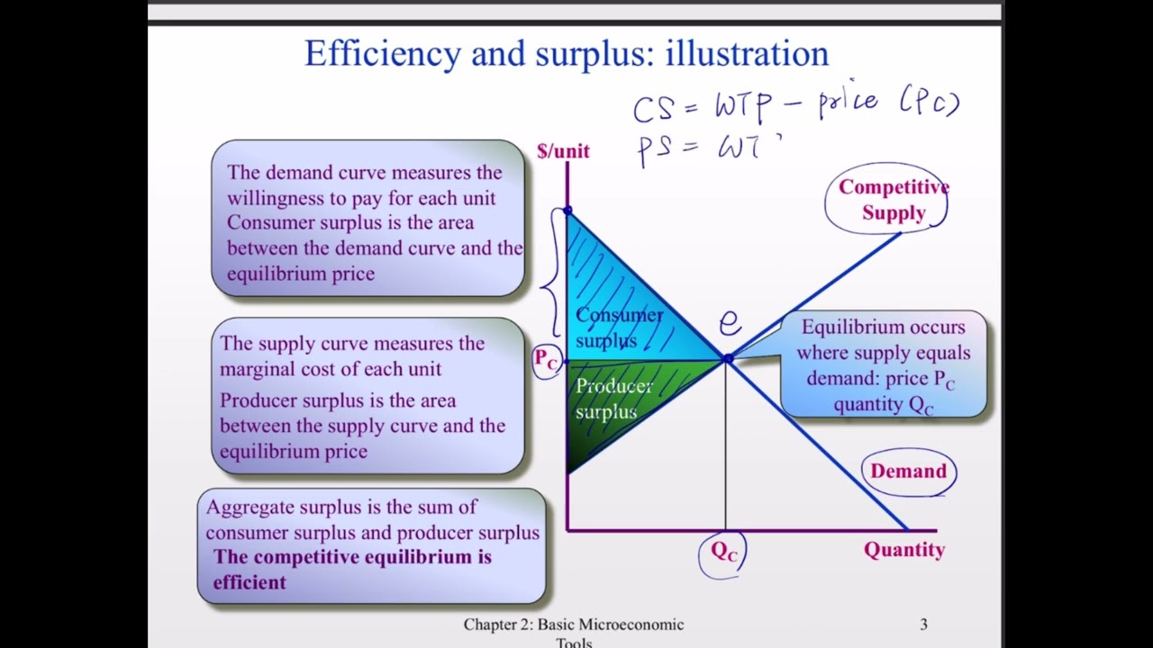
[00:48:10]Okay? Then we're going to use that market equilibrium of these demand supply curves to assess the size of the pi. And when I say the pi, I mean how big is consumer surplus and how big is producer surplus. Consumer surplus is the difference between the benefit consumers derive from purchasing a good and the price they pay for that good.

[00:48:30]Producer surplus is the difference between what price producers receive for the good and what their mar their cost of production was, what their variable cost of production was.

[00:48:40]Social efficiency is the sum of consumer surplus and producer surplus. When there is something happening such that the competitive equilibrium is not being achieved or that somehow the social optimum is not being received because there are market failures, right? There are externalities, there are public goods, etc. etc. There's loss and we call that loss dead weight loss. It's sort of the sub-optimal. Uh it's the difference between what's happening and the optimum. The first fundamental theorem of welfare economics tells us that competitive equilibrium in a well functioning market maximizes efficiency. Right? What did I say? Well function. If there are market failures this will be this will not be true anymore. The second fundamental theorem in welfare economics tells us that the socially max the social efficiency maximizing outcome.

[00:49:27]The second welfare theorem tells us that we could reallocate initial bundles to achieve any post-equilibrium allocation of resources. But like I said earlier, reallocating initial bundles is really hard, right? It's not very easy to take away someone's assets and give them to somebody else. That's not allowed in society. Because of those restrictions, we fundamentally face in economics this trade-off between efficiency and equity.

[00:49:49]In order to redistribute resources, we have to weaken incentives by taxing by uh by sort of taking right we weaken incentives to accumulate to work to invest in order to create redistribution. And so we fundamentally have this trade-off between equity having a distribution of income or resources that we like and efficiency which is having the biggest possible pi.

[00:50:10]This trade-off between how the pi is divided and how big that pi is because we really can't transfer initial uh resources very effectively. We just can't really do it by law.

[00:50:19]Okay, so let's take a look at what our social efficiency picture looks like. So we have supply and demand here. Um I said that consumer surplus is the difference between the benefit consumers demand and the price they pay. Right?

[00:50:30]The demand curve is in fact a lining up of people by how much they're willing to pay for this good. So let's say this is you know whatever good this is a can this is a can of soda. I'm really thirsty so I am and I love soda like I love corn syrup right? So I am that guy on on the on the y- axis. I get the full difference between W and X because I love soda. I'd pay much more above the equilibrium price, right? Equilibrium price is where supply equals demand. I would pay far more than that. I'd pay W for a soda. So if I just have to if I only get if I only have to pay B, it's a win. It's a big win for me. The next person, you know, the next person over is someone who likes soda but not quite as much as I do. Their willingness to pay is slightly less than mine, but again, they would pay way more than the equilibrium price, too. We're going to line these folks up until we actually hit equilibrium. Right at that point, the last person at Z is a person who's basically indifferent between buying the soda at piece of B and not having it at piece of B. That's exactly their willingness to pay. The person to the right of equilibrium, right, the person like over here, they don't buy a soda.

[00:51:32]And why is that? Because they don't value it at what they'd have to pay for it. Okay? So, and similarly, the producer surplus is the difference between what producers receive and their marginal cost of production, which is what the supply curve is. The supply curve is the marginal cost of production above the uh average variable cost right summed up over the different producers.

[00:51:51]So that the beige triangle is producer surplus. The uh blue triangle is consumer surplus. Would these triangles be bigger or smaller if these lines were more steeply sloped?

[00:52:02]Bigger.

[00:52:05]I love it. Smaller. Bigger. Yes. Okay.

[00:52:08]Um yes, it would be bigger. Right.

[00:52:10]Because what would what does Let's talk about consumers. If demand is more steeply sloped, what does that mean? It is it's more or less elastic.

[00:52:18]Less. It's more inelastic, right? It's more inelastic. When we say that demand is very inelastic, what we're really saying is that the consumer does not have good substitutes for this good, right? For me, I don't think Pepsi is anything even close to Coca-Cola.

[00:52:33]There's no substitute for Coca-Cola for me. So, my demand is incredibly inelastic. If you offer me a free Pepsi or or a Coke for two bucks, I'll buy the Coke, right? I have no interest in Pepsi. For me, there are no good substitutes for Coca-Cola. So, my demand would be very inelastic, very steeply sloped, people like me. If society was made up of people like me, if society is made up by slightly more reasonable people, right? People who found Pepsi to be a fairly good substitute for Coke, demand would be far more elastic and the curve would be flatter and there would be less consumer surplus because purchasing Coke doesn't make them as happy because there's also Pepsi, right?

[00:53:01]It's the fact that there's no good substitutes that makes demand far more um inelastic. Excellent. Okay. So, let's talk about uh oh, let's talk about price floors for a second. Um, so let's say um you know, Mayor Bloomberg really doesn't want a price floor. He wants uh I mean he he wants he wants to he wants a price floor, not a price ceiling. Uh he wants to get rid of my he wants a lower uh soda consumption. But we're going to think of an example of some other government that says, you know what, soda prices are too damn high. We're going to restrict soda prices. We're just actually going to say that they can't exceed Pab R. So the equilibrium price is PB, but this government fiat has said that soda prices cannot exceed P sub bar. So all soda will be sold at P sub bar. How how many units of soda would consumers like to buy at Pubar? All the way out there, right?

[00:53:47]Where that P bar line intersects the demand curve? They're out of luck, right? Because suppliers are willing to produce how much? Q subar. So what's not going to happen?

[00:53:57]All those units that would have been sold in the competitive equilibrium the units between Q sub and Q subb those trades will never happen. So instead we will have a market where at P subar quantity Q subar is supplied. What's the new consumer surplus going to be? Uh give it to me in shapes. Uh the names of shapes.

[00:54:17]A and what else? And what? A and B. B is in boy.

[00:54:23]Because D and E no longer exist. Right?

[00:54:25]Those trades don't happen. And that is dead weight loss. So the new consumer surplus is A and B. What's the new producer surplus?

[00:54:32]Just C. And D and E are dead weight loss because this government restriction has prevented trades that would have other would have otherwise benefited both consumers and suppliers from happening.

[00:54:43]These trades would have happened and now those units of soda are forever lost.

[00:54:47]Right? So that's dead weight loss. DNA of the dead weight loss. So what was the so part of the impact was that there's dead weight loss DNA. What happened to B? It went from whom to whom?

[00:54:58]consumers. So we changed the distribution of the pi but there was a cost to changing the distribution of surplus. Namely it was D and E.

[00:55:05]Terrific. Okay. So that's sort of you know that's sort of uh efficiency. Now we talk about welfare which is sort of our notion of equity and how people are doing. So the way we represent society's sort of aggregation of individual utility is called a social welfare function. It's how we add up the utilities of different members of society to get a measure of sort of societal welfare. We call this a social welfare function. We're going to talk about two particular forms of social welfare functions. So social welfare functions could be very different, right? A social welfare function could be like I only care about how short people feel about things, how well they're doing. They're my people.

[00:55:39]They're the only people whose utility I put any weight on. If you're over 5'6, I don't care about you. That could be a util that could be a social welfare function, right? It's not a common one, right? We're going to talk about two in particular. One is the utilitarian social welfare function in which case we value everyone equally. We just add up their utilities. I I value a unit of Matt's happiness uh equal to I value a unit of Jeff's happiness of utility. So I just add it all up. If we have a utilitarian social welfare function, it will be true that to maximize social welfare, we'll want to equate the marginal utilities of people.

[00:56:14]Not equate the utilities, but the marginal utilities. Why is that? It's not that I care about Sorry. It's not that I care about a unit of Matt's happiness and a unit of Jeff's happiness equally. It's that I mean it is yeah I I care about it equally. So I'm going to want to equate marginal utilities across people. Why is that? Suppose suppose Jeff had a much higher marginal utility of soda than Matt did or of consumption.

[00:56:37]Let's just say some consumption good.

[00:56:38]Some aggate consumption good. In that case, taking a unit away from Matt and giving it to Jeff would be a win for the social welfare function because his marginal utility is higher than Matt's.

[00:56:49]When I take a unit away from Matt, Matt is sadder, sure, but Jeff is happier for that extra unit by more than Matt is sad. So, when I'm just adding up people's utilities, I'm going to want to equate margin utilities because I'm going to want to make those trades until there's no more gain from moving around consumption, until margin utilities are equal across people. Does that make sense? Good. Excellent. The other kind of social welfare function we'll talk about is a Rouseian social welfare function. This is the case where we want to maximize the welfare of the worst off person in society. So the minimum of all the utilities is what we want to maximize. So this notion comes from John Walls's idea that suppose uh we were like at a dinner party before any of us were born. It's like some kind of pre-existence dinner party. And we were talking about, you know, how we should allocate res resources in society. And we had no idea whether we'd be princes, we'd be poppers, we'd be investment bankers, we'd be god knows what, right?

[00:57:40]We had no idea. We would be very concerned about being the worst off member of the society according to John Ross, right? We'd be very concerned about how that person would fare because we'd all have a decent shot of being that person if we had this dinner party exanty to ex to existing. That's where this idea comes from that we want to take care of the least welloff because uh you know behind the villa of ignorance that could well have been us.

[00:58:00]So this implies that social welfare is maximized by making sure the worst off person is not doing so too too badly.

[00:58:06]Simple idea under roles. Okay. So let's go back to our tanniff example. So the blue supply curve so demand is constant here. The blue supply curve is uh the labor supply of single women with no TANIF program in place. With the $5,000 benefit guarantee version of TANF in place, our supply curve is S sub2. When we reform welfare and reduce the benefit guarantee and increase work, right, we move back uh towards the initial equilibrium and we're at S sub3. So what happens to efficiency in the story when there is a lot of there is dead weight loss created by the initial program, right? When we have the $5,000 benefit, the dead weight loss triangle is abcde e. When we cut benefits and increase work incentives, these people the the single women work more and our dead weight loss is reduced to D and E. So efficiency is enhanced by reducing the benefit guarantee program.

[00:58:59]Is society better off? Unclear, right? Depends on first of all, well the women are certainly individually worse off when we cut benefits, right? because sure they're working more, their income levels haven't fully fallen, but they're giving up leisure to do that and their incomes are less. So women are certainly worse off, but maybe we value the sort of societal surplus of ABC more than we value their discomfort of working. It depends on our social welfare function.

[00:59:27]Depends on what weights we put on different parts of society. Okay, let's look at two examples. So in the we're going to actually use a we're going to look at a utilitarian social welfare function. And each individual's utility in this case is simply uh square root.

[00:59:42]So utility level is simply the square root of your consumption. We're just talking about a consumption good is some kind of aggregate measure of consumption. So u equals c to the 1/2.

[00:59:51]Suppose um the population of the poor the share of the population of poor people is 10%. And the non-poor are 90%.

[00:59:58]Okay. So with the big tan of benefit, our incomes are sort of post labor market incomes are the benefit ends up with uh the poor getting $10,000 a piece and the non-poor having $50,000 in post tax income post tax post transfer income. The average income of the society, right, is 0.1 time 10,000 because the weight on there's 0.1 uh the weight of of poor people is 0.1. The weight of non- poor people is 0.9. So the average income is 0.1 * 10k plus 0.9 * 50k which amounts to $46,000. That's the average income. What's the a what's the social welfare of the society? Well, what's the utility of a poor person here? It's 10k to the 1/ half, right? And how many of those folks are there? There's 0.1, right? What's the utility of a non-poor person? It's 50,000 to the 1/2. And the weight on that type of person is 0.9. Is that a question? No. Okay. Um, so the social welfare is going to be 211.2. Let's say we cut tan of benefits.

[01:00:56]When we cut tan of benefits, we need to le raise less revenue, right? There's less stuff we're spending money on. So we can actually reduce taxes. It's going to change post transfer post tax incomes for these two groups. The poor now are only getting $5,000 a piece in the society. The non-por they're not paying as much in taxes. So they're each getting $51,000 a piece. So what's average income in the society? Well, it's going to be 5k * 0.1 plus 51k * 0.9. Average income has gone up to 46,400. Let's look at social welfare.

[01:01:26]So, what's the utility of a poor person now? It's 5k to the 1/2 and there's 0.1 of them. Uh what's the utility of a non-poor person now? It's 51k to the 1/2 times 0.9, right? That's the weight on them. So, our total social welfare is 210.3.

[01:01:42]So even though average incomes are higher because we've strengthened the incentives to work for the poor and the non-poor, right? We're taxing the non-poor less. We're sub we're um giving smaller benefit guarantees to the poor.

[01:01:52]So everyone has stronger work incentives. Average incomes have gone up. But society according to this social welfare function is not better off. How could we have how could you have told me that before even doing this calculation that if we change incomes in this way, people won't be better off at the income levels of 10k and 50k.

[01:02:10]Who's notice that they have the same utility function, right? They don't poor and non-poor not fundamentally different. They value consumption according to the same function. So if the incomes are 10k and 50k, who has the higher marginal utility? The poor, the non- poor. The poor because they're consuming less, right? Marginal utility falls as we consume more and more, right?

[01:02:31]Diminishing marginal utility. So you could I you could have told me that if we uh take income away from the poor and give it to the non-poor, we're distributing redistributing from someone who has a high marginal utility of income of of consumption to someone who's a low margin utility of consumption. So we're guaranteed to not be better off for sure. When we trade that in that direction, we're going to have a lower social welfare. Why is that? Because this is a utilitarian social welfare function. We're making trades away from high marginal utility people towards low marginal utility people. We're going to be worse off. And that's because this society is somehow a utilitarian society. It's it's got this particular functional form for social welfare. A different social welfare function could come up with a different a different um a different uh welfare consequence. So for example, um in scenario two, so different assumptions can have different effects. So it's very simple for me to say if our social welfare function were different, we'd have different out we would have a different outcome. Like if we had a social welfare function where we only cared about the non-por it would be pretty clear, right, that we would be better off and when we cut welfare benefits. If we had a social welfare function where we only cared about the poor, it would be clear that we would be worse off when we cut benefits, right?

[01:03:38]So let's not mess with the social welfare function. That's a copout. Let's make other assumptions about how this change in the benefit structure affects incomes. So let's say that the disincentive to work for the rich of being taxed so much to pay for that benefit was really high. Let's say in fact when we cut benefits, sure the poor are still going to get $5,000, but because they're being taxed less, the non-poor work a lot more. They in fact have $55,000 of income. In this case, the labor supply response of the non-poor is so big. They make so much more money that society is actually better off because um average income has gone up to 50,000.

[01:04:19]we have the same uh so that one half should be um sorry those should be superscripts it should be the same utility function so the the utility of a poor person now right is 5k to the 1/2 but the utility of a non-poor person is 55k to the 1/2 because they worked a lot more because of the reduction in their taxes right they earned a lot more in this case with a different assumption about the responsiveness of the non-poor to taxes we end up with a society that's actually better off for having cut benefits does that make sense um So in in this case um because the income increase that the non-por experience from having lower taxes lower disincentives to work is so large that societyy's actually better off for the benefit cut because I said transferring so let me go back for a second I sort of misspoke earlier transferring income from the poor to the non-poor right is sort of we're making trades from high margin utility people to low margin utility people but in this case the increase in income that the non-poor earning is so big it offsets sets the fact that we're trading from high margin utility people to low margin utility people. The increase in consumption is so big for the non-poor it actually society be to be well off.

[01:05:27]Is anyone confused? I sort of misspoke earlier. It's okay. It's my fault if you are. Anyone want me to say it again?

[01:05:34]Let's say let me say it again. So in this case here we know that we're transferring money from someone who's high marginal utility to someone who has low marginal utility. Right? We're going from reducing the consumption of the poor, increasing the consumption of the non-poor. Whether or not society is going to be worse off or better off when that trade happens depends on how much more income is in this pie. Right? In this case, we cut the benefits of the poor by 5,000. We increase the income of the rich by a thousand. There are a lot more rich people, right? There's nine times more rich people, non-por. So, it could be true that society is better off, right? But in this case, it happens not to be because the increase in consumption for the low marginal utility guys, the non-por is not big enough and they're not enough of society to offset the fact that the marginal util the reduction in consumption of high margin utility people was so big. Right?

[01:06:26]Societyy's worse off here. In this case, in this another way to think of this is that changing the distribution of the pi didn't increase the size of the pi enough for society to be better off in this scenario. But in a case where the non-poor are far more responsive to tax cuts, right, they're working a lot more, the fact that we're taxing them less is growing the pie to be much larger here, right? They're earning a lot more income. This means that even though we're still making the trade from a high marginal utility part of society to a lower marginal utility part of society, the increase in consumption for the non-por is so big, it's 5k here, that we're actually better off as a society.

[01:07:04]We grew the pie enough that the fact that we're redistributing this way didn't still led us to be better off.

[01:07:10]Does that make sense? Uh Eric with a K.

[01:07:14]Yes. So that's doesn't make a silly comment. So that's why it's better to um tax the rich less than 15%. It makes the pie. It depends. Um so you know if that were true I mean maybe it's true. I mean it's an empirical question right? If if uh you know if so so in the US we'll talk a lot more about this. uh investment income is taxed a lot less than than earned income and that's partly because capital is mobile right you can go abroad can be invested elsewhere so if the fact that society is under capitalized is costing us so much productivity that we're better off reducing taxes on investments so that people invest here in the US it could be true that even though people who tend to hold capital people who tend to be investors tend to be on you know for by an empirical fact tend to be wealthier than people who derive most of their income from labor um that if you're a utilitarian you may not feel really great about that redistribution in that sense. But it could be true that the productivity effects of having more capital invested here in the US could offset it. The pi growth could be bigger. It's an empirical question.

[01:08:10]Theoretically, there's no, you know, this is not going to we're not going to get there with theory alone.

[01:08:13]Historically, um we Yeah, I said it's an empirical question. So, we're not talk I mean that's a whole other set of lectures.

[01:08:19]We're not we're not going to get there.

[01:08:21]Um okay, terrific. Okay. Empirical tools of public finance. So, that's all of the theory. Like I told you, there's nothing I talked about today that you haven't seen before. Micro, right? You're not going to learn a lot of new theory, but you're going to apply it in weird and different ways. Uh fun in different ways. Fun in different ways. Okay, terrific. Okay, so let's talk about empirical stuff. We're going to go through this relatively quickly. We may not finish all of it. That's okay. You can always uh the problems for homework are doable if you read the chapter. But okay, empirics. So empirical public finance is all about estimating the size of indirect effects. How big are people's responses in the direction that theory predicts they would respond? Do they respond? How big are the effects?

[01:08:58]So fundamentally empirical public finance suffers from the identification problem. This is the notion that if two variables A and B are correlated, we still don't know exactly how their causal relationship or what their exact causal relationship is. For example, um it could be true that um I gave this complicated example during the day class. We can do it again. Suppose we see that people who use asthma inhalers tend to be have better running times than people who don't. Right? Is it that asthma inhalers are causing people to be faster runners?

[01:09:29]It could be. It could be that people who are really into running fast sort of really look into the, you know, the the whatever benefits they could get. So, they already would have been fast and they use inhalers. It could be that the people who have the resources to go to the doctor and be diagnosed as asthmatic also can afford better sneakers and so they're better faster runners and they're more likely to have an inhaler, right? Um that so those are our separate those are things, right? It could be that the inhaler is actually causing people to run faster. It could be that faster runners sort of care about every edge they can get, so they actually go out and get inhalers, right? It could be B causing A. It could be that there's some third factor C sort of income levels that's causing both A and B, right? It could be any of those things. So, we want to sort this out. We want to figure out is A causing B. The gold standard of research in empirical public finance in most empirics is the randomized trial. Randomized trial means that for each of you, I go around the room. For each of you, I flip a coin. If it's heads, you're in the treatment group. If it's tails, you're in the control group. And if it's heads, I, you know, give you an inhaler and make you take two puffs of it. Right? This is a randomized trial. Half of you get aluterol. Half of you don't. And then we go out to the field and you run and we time it. That's a randomized trial. It's the gold standard because what's the problem with suppose some of, you know, I I use inhalers. So, some of us use inhalers, right? The fact that I use an inhaler is may or may not affect my running times, but it's certainly correlated with many things about me, right? It's correlated with my income level. It's correlated with my education level potentially that I know that if I'm having breathing problems, there's some solution to it. It's correlated with my interest in exercise, right?

[01:11:05]Maybe if I never exercise, I wouldn't know I had asthma, right? It's correlated with so many things about me that you can't really disentangle the two without randomizing. Because when you randomize, what determines whether or not I got an inhaler today? A coin. Nothing about me. Nothing about my income, nothing about my exercise preferences, nothing about my shoe size, nothing about me is determining whether or not I I I I used inhalers today. That's what randomization does is it sort of creates a treatment and control group that in all other respects besides the treatments are statistically identical.

[01:11:38]There's no reason why uh one group is poorer or richer than the other as long as the group is big enough, right?

[01:11:43]There's no reason one group exercises more than the or the other. The coin didn't know anything about you, right?

[01:11:48]So that's why randomized trials are the goal stand, but there's lots of issues with this, right? Like first of all feasibility. So maybe with this inhalers and running times thing, we could maybe do this. But something like uh you know macroeconomic problems. We only really have one macroeconomy. We can't really run randomized trials on the macroeconomy, right? Some just too big a um a system to actually randomize it.

[01:12:11]Second, ethical concerns. So, I'm guessing that Wagner probably would not let me do this, right? NYU has a standards bureau and they probably wouldn't let me pump aluterol in some of your lungs and not in others lungs and see what happens. I mean, let alone the lack of education, it would probably be unethical, right? You could have side effects and do we really care about this question, etc., etc. There's ethical concerns. There's threats to internal validity. So, um, when you run these types of trials, like you can't typically mandate people stay in your trial. So, suppose you do we divide the room, this side gets the inhalers. Some of you have some bad reaction to the to the to the inhalers and you know you uh you stay in the room and you don't somehow I miss the fact that you're not on the field with us. It's not random who's going to have a bad uh it may not be random, right?

[01:12:55]Who has a bad sort of reaction to albuterol, right? It could be people who are weaker lunged to begin with and are just thus slower runners in general. And so it's going to make the inhalers look better than they are because the population of people who use the inhaler who actually runs the race is different than the than the entire treatment group. Right? This is called attrition.

[01:13:13]My silly inhaler example is silly. It's a real problem with something like let's say charter schools, right? So suppose we have a lottery, right? And we actually lottery kids into charter schools, randomized trial. We're totally psyched. We're going to, you know, have a great sort of clean experiment published in a great journal. We're all very excited. But then some kids when you they enter the charter school have a a rough time. it's not working for them, they are likely to, you know, not the kids it was working really well for who are likely to drop out of that school and go to a different school. It's the kids who it wasn't working for. So we may see them drop out of the whole system. They may go into the private schools or they may drop out of school period. Right? So the sample that we get outcomes on may very well be different than the sample we randomized the group we randomize people into. And that attrition is unlikely to be random. It's unlikely to be random. It's going to be some sort of selected group that doesn't make it through to the outcome. So attrition is a real threat to what we call internal validity. That even within the people who are subject to the treatment and the control, we may not be assessing the average impact correctly. More broadly, we have threats to external validity. Right? Our sample may somehow be unrepresentative with our inhaler running times trial. Who am I doing this to? The people I can, right?

[01:14:20]My students. You guys, are you really representative of most New Yorkers? No.

[01:14:25]Right? You're clearly well you're clearly more educated than average. You are eagerly here. brighteyed and bushy tailed, right? You are somehow afraid of me enough that you're comp you're cooperating in the study, right? These are not things true of most people. And so the external validity comes from the unrepresentiveness of the sample. This could be that you know the cities which let you run charter school lotteryies may not may be more progressive or more research-minded than the average American city. This the people who live there may be slightly different than people who live in other cities because of that. Right? there are various things about the places we're allowed to run studies that may be sort of different than the than society at large. So that's external fluidity. Okay. So what are our empirical tools? So we're going to first talk about time series regression. Um so time series regression is the idea that we're going to analyze the co-movement of two series over time. So for each date we have a one observation of these two um series you know whatever they are and we're going to see how they're related over time. So let's look at this. The red line is the average hours of work um by single mothers each year. The green line is the average monthly benefit guarantee for a family of four. So what would you say, you know, if you naively looked at this, you would say, hey, it looks like monthly benefits go down, right? And labor force participation or hours worked, not participation, but uh hours worked seem to go up. So naively, you could think, yeah, you know what? It seems like one goes down, the other goes up. They're negatively related. cutting benefits increases uh labor supply. But this is a long period of time, right? 1968 to 1998. Was the only thing that was were were there other factors besides welfare benefits changing during this time that could potentially affect uh the labor force choices of women? Yes.

[01:16:10]Sorry.

[01:16:12]Yeah. More work opportunities, right?

[01:16:13]This was a time where technology was changing. There's a lot more home technology, right? Maybe women were more able to sort of leave their their traditional roles and work more, right?

[01:16:21]There were changes in um the equal rights movement that allowed women to earn more for the same work, right? That made work more um made work higher return for women that could have changed uh hours worked. There um were changes in other policies as well, right? During this time in between the late 90s and between the mid 90s and now we we greatly expanded a program called the EITC which is sort of a wage subsidy program that clearly probably affected labor supply um of women starting in the 90s and is is not in these are all confounding factors right they affect labor supply in ways that the monthly benefit guarantee is not fully capturing another thing that happened is there's a huge there's a business cycle right there was a general growth this was generally a period of growth you can actually see in the 90s we know the 90s were period of very strong growth You can see labor force hours were work hours were going up very steeply there.

[01:17:08]Another sort of telltale, right, is that there's there are subsets of time where these two things are not negatively related, right? We could look at um benefits are sort of going up in the first couple years and so is average work hours, right? This isn't everywhere true and it's more or less true in different periods. So this sort of wobbliness of these two series suggests that you know what they seem to both be kind of declining in some general sense or in one is declining other is increasing but in this very general way right there's nothing sharp in a time series for time series evidence to be compelling what we want to see is sharp changes in one series and sharp changes in the other series that are contemporaneous or have some kind of fixed lag to them right that it's always happening a year after something we'd like to see sharp changes and hopefully multiple changes right where one picked up suddenly and then picked up again later and we see the same pattern in the other series that that contemporaneously or in some kind of um fixed lag period.

[01:18:05]There's some structure to their relationship and we see it in sharp changes. For example, your textbook talks about an example with um cigarette prices and teen smoking. That's a very sharp change, right? There's two changes. There's a time when prices went down because of a price war and time a time when prices went up because of um uh the tobacco lawsuit. and we see sort of sharp changes in teen smoking behavior in the directions we'd predict at both of those times, right? That's compelling time series evidence. It's not that time series is never good. It's just got to be very compelling uh for us to really believe. The second uh empirical tool we'll use is cross-sectional regression. This should say two, not three. Oh, no, this is three. This is three. This is three.

[01:18:45]Sorry, this is three. Is cross-sectional regression. So cross-sectional regression is the analysis of variables across people within the same time period. So this would be, you know, me asking you how tall you are and what your grade in micro was, right? You're different people and in the same period of time I'm asking you questions about uh we're comparing across individuals the same period of time. So in our tanniff example, we could try to run a regression where we look at the hours worked by different women as a function of the benefits they receive employing some set of controls, right? Because so what is the problem here? Suppose I just looked at um tan of benefits and uh labor force hours. What if you know benefits vary by state, right? And different like right now different states are fairing differently in this economy, right? So it could be true that a state that is not doing well, right? has low work hours by women because they're particularly hard hit by this recession and they can't afford a lot of benefits, right? That would give us the opposite relationship that low benefits and low and low work hours go oh yeah and low work hours go hand in hand, right? But that's not really about tanniff and how it affects labor supply. That's about how there's a variable C, the recession affecting both of those things, right?

[01:20:00]So we could try to employ controls. We could add a control for the state unemployment rate um the unemployment rate in the state the woman lives and that takes care of that but you know there's also just fundamentally preferences right people are different the same benefit may you know I may really love law and order right doesn't matter what my welfare benefit is I'm not going to work that's going to give us that's a confounding factor right my personal feelings about leisure versus uh consumption are going to affect the way tan of benefit changes change my hours worked so even if we do unemployment rates and we do industry decomposition and we do 50 things, we're fundamentally never going to be able to control for the preferences of individuals that differ across people, right? What I mean by that is there's always an X factor that no matter how much data we have, we can never really control for the individual fixed characteristics that are unobservable that affect both our TANF recipency and our work hours. Does that make sense? And this is why cross-sectional regression is dangerous. when I comp when I ask you guys questions about, you know, how tall you are and how well you did in micro, it's less true here. This is America.

[01:21:04]It's a well fit society. But if we look at um suppose we we're trying to do an analysis of the returns to height in an area of the world that has had very high rates of famine or poverty, right?

[01:21:15]That's not going to be the returns to earning of height, right? It's going to be was your family poor. Maybe a poor family both has shorter children because they're more affected by famine and couldn't afford education, right? That's not going to give us a causal interpretation of the effect of height on earnings if there are factors that we can't control for that affect both. It could also be that you know some families take better care of their children and are more apt to feed them properly and more apt to give them the skills that lead them to earn more. And we can try to control for you know the income of your family, the education of your mother, the height of your father.

[01:21:48]You try to throw all that in. We'll never fundamentally get to the family preferences, right? We're sort of trying to get it out. we're never going to get to act with the X factor. So all cross-sectional regression is potentially confounded by individual fixed characteristics, right?

[01:22:00]Differences in preferences, differences in sort of spunk, right? And that's going to fundamentally sort of um make cross-sectional regression difficult to interpret. So this is an example of a line from a textbook. You can go ahead and read this on your own. I want to get on to uh oh, you know what? We're already over. So we'll talk about panel data and quasi experimental methods next time. Um, do read it in the chapter this week and we'll just talk about it next