Ghost and Stray Light Analysis with TracePro Tutorial

[00:00:00]This is Mike Gobin and today we're going to uh I'm going to introduce you to how to do ghost and stray light analysis using tracero. So first of all in this webinar you will learn how to use trace pro to analyze ghost paths. Learn how to understand and use important sampling for scatter analysis. Learn how to understand and use tools to analyze stray light issues.

[00:00:25]The current Trace Pro release that uh you should be using is Trace Pro 7.1.2.

[00:00:30]If you're on the current release, you can download this uh and it is available to anybody who's underneath the current maintenance and support agreement. And of course, the website's www.lamarez.com. First of all, rate tracing for optical simulation. How does this all work in Tracepro? Well, first of all, if we have no optical constructs except for the block and the cylinder that you see here, you need to create a realistic virtual 3D model and we have solids. So, in other words, what you're going to have is two objects in Trace Pro. And then after we've made these two objects in Trace Pro, we can apply surface and material properties to the model. We can create a source and launch light into the model. And then we let Trace Pro determine where the light goes.

[00:01:18]So pretty much what happens here is that five things can occur when light hits the surface. If we take a look on the left hand side here and we see a ray coming in, it can do multiple things.

[00:01:30]Five of them. As a matter of fact, it can refract off the surface. I'm sorry, refract through the surface. That's this red that you see going through here. It can reflect off the surface. There's the black surface for that. It can absorb right on the surface. It can scatter as you see over here in this diagram. You see all the scatter going on here both in a forward direction and in a backward direction and it happens at each surface. This doesn't even figure in the volume effects that are possible for trace broke to use. And we keep track of all this in terms of the flux, the ray direction and the power and we report it in the flux report.

[00:02:11]Let's take a look at the material property definition. What happens to an incident light ray? Well, it's going to refract as it hits the medium. The medium right now is this top surface over here. And the light refracts as it goes through. And we follow Snell's law. So pretty much what happens here is that we define light rays instant to a boundary between two mediums like plastic or glass and air. The light rays are refracted to this boundary and this shows the interaction. So light is bent and as we noticed as we go through here the angle that comes into the particular object comes out at that same but it's shifted because of the refraction and it follows Snow's law which means that the formula that you see over here NI sin theta I= NF sin theta F or is that R I'm sorry sin theta R is the angles that are involved as the light comes through here and that's what causes the bending that you see in this particular slide. Well, at each one of these surfaces, there is some Fresnel loss which happens when light rays cross from one refractive boundary to another. So, pretty much the amount of frenel loss is calculated by using the formula you see in front of you, NI - NF over NI + NF squared. And so pretty much for a a plastic or say a BK7 we're going to lose about 4% on any surface 4 to 5%. And this for now loss is not much when you think about it for a visible type system. But when you have six lenses that's 12 total surfaces at 4% loss.

[00:03:54]You've just lost 50% of your energy. And in an infrared system this renell loss is much higher. So usually this is why you have to anti-reflection coat a lot of the lenses or you're going to lose quite a bit of your energy as you go through the particular system and trace keeps track of all this. So in terms of this we now have refraction we know what happens on all the surfaces but then when we add in total internal reflection in this case this is something that we want in a lot of systems because trir occurs and there's no fresnel losses. So what happens is is that there's a critical angle and the critical angle is defined right over here by sin theta f at 90° equal to 1. This then reduces snow's law to this simplified equation. And so when we look at something like plastic, the critical angle is about 42°.

[00:04:47]So what happens here is that when we have a critical angle hit about 42° there you see a critical ray coming off and it has 100% of the value of the energy that it started with. So there we can see what happens when we actually refract and then we hit the critical angle and it actually reflects right off of that particular boundary. And of course this is something where the rays start in the media and they hit air so that we understand what the NF and NI index refraction in the media and not and incidents in the media are. So how does this all occur in terms of trace bro? Well we use a generalized Monte Carlo ray tracing algorithm inside the program. It's nondeterministic. The ray trace has multiple choice points. Each choice is determined by a pseudo random sampling of the probability. A good sampling requires many rays. So when we look at something like an LED and we want to talk about all the different angles that we might want to look at in terms of how that LED is going to go through a lens, we need a lot of rays. Around 10,000 is a good sampling amount. For that reason, when we're looking at things like scatter or things of that nature and we want to look at a certain area, we want to make sure that we have enough sampling points in that particular area.

[00:06:02]And Monteol ray tracing allows us to do some of this. Rays can be split at choice points. Splitting or not splitting is available in trace pro so that you can get very accurate results.

[00:06:13]But if you want faster rate trace times, you may want to use something like important sampling. So low probability paths may be undersample with traditional Monte Carlo methods and important sampling helps us increase the sampling in those low probability paths.

[00:06:28]I'm going to talk about that uh pretty soon here as we get through this uh particular slides. Well, let's start off with something that um you've probably run into which is ghost analysis or ghosting in your system. And pretty much a definition of ghost is that ghost images are out of focus images of bright sources. Light must reflect an even number of times from lens surfaces. If the source is small, each ghost looks like the aperture stop. If the ghost is focused on the image plane, the ghost looks like the source.

[00:07:06]So a complex ray trace example with a flux threshold set of 0.00001 means that we're going to have light that is going to hit this lens over here. So we have an incoming set of red parallel rays that strike this surface here. And in this case what we see is that there are a lot of blue rays coming in throughout this particular system.

[00:07:32]The ray splitting happens due the fresnel losses. So all these rays are hitting the front surface and they're coming off the front surface. And that's where you see this focus over here of these rays hitting that particular surface. If they come in and hit the back surface and then hit the front of the first surface. So here's your double reflection and then come back through, you get the focus over here.

[00:07:55]So decreasing the flux threshold in the rate trace options allows us to see these ghosts because as you know it's about 4% per each surface and if we multiply 004 * 004 we get 0.16 as the amount of these blue rays that are coming forward and if our flux threshold isn't low enough we're not going to see these ghosts. So the first thing that we need to know in the ray trace options is that if we want to see ghost of this magnitude with double reflections, we need to set our flex threshold a little bit lower than the 5% default that's usually in trace pro.

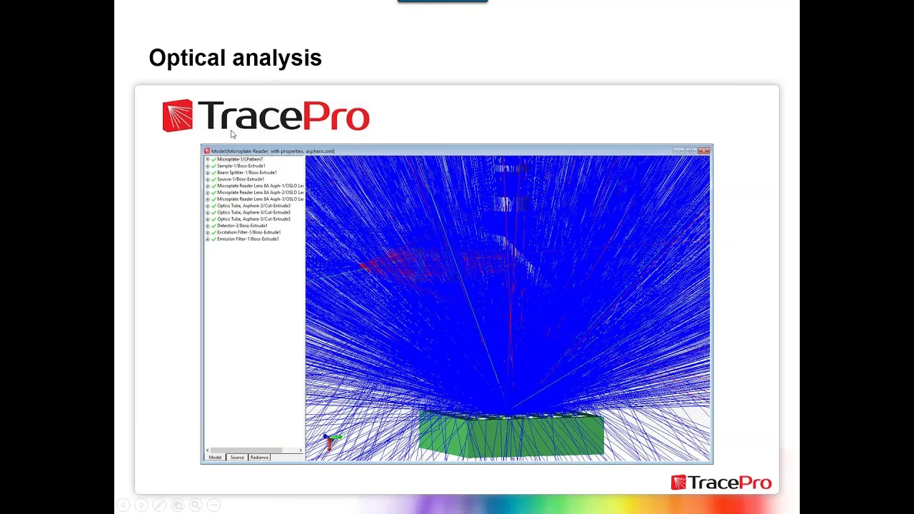
[00:08:29]That's when we're going to be able to see this type of setup inside the program. So if we look at every single path that actually can occur in this type of system, here's your parallel set of rays coming through. There's your lens. And there you see a couple of rays. The two blue rays here. That's the particular selected ray path that I have shown here in Trace Pro's ray path sorting. Ray path sorting is new in Trace Pro 7.1. If you go to the analysis menu and you look up path sort table, it's going to create this table for you.

[00:09:10]And you could say that there are a number of paths. And each one of these paths is numbered by trace pro. And if you click on it, which I have done for the first path and the second path, and then use the capability to say analysis display that selected path, it will then show you the rays for that those particular selected paths. So in this case, ray path one. Ray path one has 99.98% of all the power coming through this particular system. Those are the red rays that you see here. Because by default, Trace Bro shows rays by their flux. Rays with high flux 66% of the starting value and up are shown in red by default. And those rays that are less than 33% are shown in blue. So that's what you see here is the blue rays. If we see over here, this is path number two. We can see that light is emitted.

[00:10:05]It then hits the front of the first surface and that's the first surface of the lens, the back surface of the lens.

[00:10:13]It then specly reflects. You see the specular reflection right over here in terms of the intercept type, the front of the lens and then specly transmits through the back of the lens and then hits the reflector and then to the target surface and it has 1% of the energy. So this path is shown as blue rays and there are two rays in that particular path.

[00:10:35]How do I know that? Here's my number two right there. The number of rays in the starting path are shown up here. So each path has information in terms of what its wavelength is, the number of rays, the absorbed flux, and this is just as we go through the columns, percentage of the total, the incident flux, the total amount, percentage of the total for that particular ray path, what the path type is, and this is specular. And you can see that each one of the surface it hits is then described underneath that particular section. It tells you how the intercept type was. Is it emitted, transmitted, reflected? And then which objects are actually hit and what surfaces are reflected or transmitted through for that particular path. So this case we have the capability to look at every single path, see where it focuses. And this is important. Is it focused right on our signal or is it off the signal? So, this is important sometimes to make sure that if we have a source uh and then that source has a ghost on top of it, how much the ghost is going to actually affect our image.

[00:11:45]And so, we can see all this path by path or multiple paths as selected in the path sorting.

[00:11:54]So if we look at a cook triplet which has a total of six lenses, we can see something like this when we ray trace it. So if we set the flux threshold to 0001 and we show all the rays, we can get quite a few different ghost paths.

[00:12:12]The ray sorting capability is quite helpful when trying to see these ghosts because in the ray sorting right now we have it set to all rays and I'm only showing 10% of the the total race since I don't want to fill the whole screen up.

[00:12:25]If I then say and put ray sorting on and say only show me the rays that actually made it to my detector, we see the image we have down here on the bottom. And this only shows us the ghost paths and I've taken out the in this case the signal. Now what's nice about tracero is that when you use the path the ray path sorting along with the radiance map, you can use them in conjunction with each other. In other words, I can show the rays for a particular path that I've selected. This is path number two. I can see how the rays actually progress through the system in the path sorting.

[00:13:06]And you can see it step by step over here. We can see that that there's reflection off the back surface of the third lens. There's the specular reflection right there point uh that's uh occurring over here. And then specular reflects off the front of the surface and then comes back through. And we can see the contribution of this ghost directly all by itself when I bring up the radiance map. So this is a way to go and click on every single path in your path sorting table and then have them show up visually in your trace pro model ray traced and then shown for its individual contribution in the radiance map.

[00:13:45]So, if you're interested in finding out exactly how rays and power is going through your system, you can use this method to see all three things at the same time in Trace Pro with these tiled windows. Now, if we coat all the lenses with a three layer AR coating, you can see that almost all of our ghosts go away. In fact, where our flex threshold is currently set, we actually get no ghosts to our detector for this particular case. And 100% of our energy actually gets to the detector now that we no longer have ghosts at this particular flex threshold. We can see that now once again we have these trace pro windows tiled and the total amount of power is 100%. And it goes right from the left to the right. There's our signal and there's our signal shown in our radiance map. A nice perfectly focused beam. Well, now that we've got through ghosting, we can look at the Monte Carlo method, ray splitting, and important sampling and really understand how trace does stray light. In Monteol ray tracing, you need to know if you traced enough rays to get a good answer. So, we're talking about sampling.

[00:15:09]A crude Monte Carlo calculation is the simplest form of a probability experiment. This is just like rolling dice many many times and counting how many times a number one comes up or a number two or a number three. Now an estimate of the probability is the number of times you throw the dice divided by I'm sorry how many times the number one comes up versus how many times you do the experiment. So in other words, if you throw the dice six times and a one comes up only one of the six times, then the probability is 1 over six or one sixth the time. We can never get an exact value of the probability estimate. But if you do it enough times, you should get a very good idea of how many times that's going to occur. Say we throw the th the dice a thousand times.

[00:16:03]Well, how many times did the number one comes up? Well, it's going to be once again how many, you know, you're going to be counting as you go along. Is it going to be exactly one sixth? Not most likely. It'll probably be one or two uh throws either above it or below it. But as we throw 10,000, these numbers should be coming closer and closer to the absolute probability. And so if you look at these particular equations, this is exactly what's happening here. The absolute uncertainty is equal to the square<unk> of p * 1 - p over n. The number of times you do the experiment. The relative uncertainty is 1 - p over p * n. So hence the accuracy of the result is inversely proportional to the square root of the number of trials. Enough trials will always lead to the correct answer.

[00:16:54]So when we look at this, we're saying hm the result is inversely proportional square root. So if I have 10% probability of getting a right answer, how many more rays do I have to to cut that probability in half to make it closer? I have to do the square of that number of experiments to actually bring that relative uncertainty down. On a higher level, Monte Carlo is a technique of numerical integration for complicated multiple integrals that cannot be done by more conventional numerical methods. So when you look at the integral that represents this type of sampling process, the variables X subi I'm sorry X subjuting G for the set of samples and repeating this process n number of times and summing the terms to obtain the estimate which is a histogram method or trapezoidal rule or Simpson rule, etc. to figure this out. You could then specify this type of sampling. So what we do in trace is Monte Carlo. We either think of it as rolling the dice or throwing as many rays as possible and having it go through system to a target. But how good our probability is going to be to give you the correct answer completely depends on how many rays we trace. As we've noticed, when you look at a system and you trace 10 rays, your detector may only have one ray hit it and in only one area, but as we trace 10,000 rays, it fills the detector and we start getting a good idea where there's no areas that don't have any rays hitting it and we start feeling more certain that we're getting a correct answer. So, how many rays should you trace to get the perfect answer? Well, as you see from here, millions and millions of rays will do that. But of course, we don't want to wait forever to get an answer. So, we're going to use this type of thing to look at what you can do in Trace Pro. Well, in Trace Pro, there are variance reduction techniques. Variance reduction techniques are used to reduce the variance or uncertainty in the results of a Monte Carlo calculation after a given number of trials. Conversely, the number of trials needed to obtain a given uncertainty can be reduced. Well, ray splitting is one of these variance reduction techniques. So, when we do things like I'd like to go and sample an area for scatter, I may trace one ray and of course I'm looking at it from a far distance off, I may not get any rays whatsoever to my detector. But as I specify that I want more splitting or more rays in my splitting, I'll probably get rays in that area. Now important sampling allows us to specify targets that we can send these scatter rays towards and usually that means we are definitely going to get rays in that area but we're also probably going to have to reduce our flux threshold because as we ray split the flux of the rays reduce. So ray splitting is a technique in which a ray that strikes a surface can be split into several component rays. And we talked about this earlier in the seminar about five different things that can happen here. Absorb, reflect, reflectively scatter, specly transmit and transmissively scatter. So the flux of the incident ray will also be split. So in other words, we keep energy conservation in the program. If you have one watt going into a lens, you're going to have one watt coming out of the lens or at least uh hopefully absorbing, reflecting, scattering, transmitting, and transmissively scattering. And each one of these rays will be aortioned the amount of flux depending on the surface scattering property, the transmissively scattering property, the spectral reflection, the transmission, and the absorption that you've put on that particular surface.

[00:20:40]And it's all according to the properties of the surface as you've set them. The process of spling is repeated at each surface intercept. So that treelike structure of rays result. This process tremendously improves sampling in most cases with a torible slowing of the ray trace. But you may be creating millions of rays. There are two modes in trace bro. There's analysis mode and simulation mode. If you're ray splitting, we're keeping track of all those splits in memory. So, you may run out of memory. And someone said to me, well, why can't Trace Pro tell me when I'm going to run out of memory? Well, the reason is is that Windows is doing your memory allocation. And when you get out of your virtual page area, it's constantly trying to free up memory. And there's multiple old different programs running on your system. So, it's very difficult for our programmers to figure out when you're going to run out because you're going into the virtual page size.

[00:21:34]There's other systems being run and background processes. So sometimes you may get into a portion where you're running out of memory. If you see that, well, you can look at this both in the task manager in Windows and there's also a nice little rate trace history report that shows you how much memory you use on these particular ray traces. You can monitor that. And if you get into a problem where you're using up too much memory, instead of using analysis mode, we have a second mode called simulation mode. that instead of keeping track of all the rays on all the surfaces in the model, we only do them on the surfaces you select as exit surfaces. Therefore, we use a lot less memory in that mode.

[00:22:11]And we've actually traced a billion rays uh in that mode without any problems whatsoever. Well, let's take a look at the ray splitting that that actually goes on here. In analysis mode, we have this incoming ray and it's going to reflect off of it about 4% if this is a u a visible system and it's going to have 96% of its light transmit through.

[00:22:31]And it's going to happen at each surface as we go through here. And you can see the progression of the light as it goes from red, which is from 100 to 66% of the starting flux, green, 66 to 33, and then finally to the blue where we're below 33%. And so here's what happens in terms of the ray splitting that one ray can do. And look at all the rays that come off of this particular lens. We keep track of all those in trace pro.

[00:22:56]And you can actually look at those as a different path in your path sorting. So important sampling is used to improve the sampling of random events without dramatically increasing the number of rays started. It uses the scattering distribution function as a probability density to aortion a fraction of the scatter ray flux into a desired direction. Important sampling can be used for emitted scattered and defracted rays only on surface sources, scattering surfaces, defracted surface and bulk scattering objects. You can also apply important sampling to bulk scatter and you apply to surfaces for all others. So in other words, we can do important sampling on sources and we can do important sampling on scattering surfaces.

[00:23:43]Okay? And what happens here? Well, we have an incoming incident ray that comes and strikes the surface. When it hits the surface, there is a specular reflected ray that comes off that usually has most of the power. But say we had an eye or your instrument sitting up here to register how much energy is coming off in that scattered area. Well, I could put a target, an important sampling target over here, and I could say, "Show me array, even if I only have one ray, set up an important sampling target, and send array in that direction, and tell me how much power will be in that ray, and show me what the delta area is going to be for that particular area that I'm looking in terms of a source target." Okay, so this is my important sampling setup in the program. What you do is you go to the surface, you rightclick, you say that you want to imply a important sampling target on that. You specify the size of the target. You specify how many rays you want to go in that area. It's pretty much that simple. So if we look at the total amount of area that all the rays could go into, it may look something like this curve over here. How big is my important sampling target? Well, it's this area right here.

[00:24:53]So if we looked at the important sampling flex over here, here's our BSDF or probability density function. Here's our our delta area that it can go into.

[00:25:02]And then my important sampling theta over here is going to be equal to the theta incremental and the integral of the BSDF time the cosine of the angle time the delta angle of this area. And so pretty much it's TS is equal to the integrated over the hemisphere B SDF time the cosine theta time delta omega. So let's take a look at that same lens as light comes through and we can see over here that we have a ray coming in. So there's several rays. So here's a ray down here coming through and there you can see that there is some forel loss going in this direction off of here. There is some random rays coming off and there's some speckle rays. Here's your speckle ray coming off that's refracted. And here's my important sample target area. And we can see all the blue rays coming from the different incoming rays in these three areas that are now sent towards this target because we've set it up. Now, does it have the important sampling area have a lot of energy going to it? No.

[00:26:07]It's all according to this formula right over here. And if we look at this in terms of the important sampling example that we have, we can see that's not going to be a lot of energy. I'm going to get into that shortly. We can do the same thing for a source example. For instance, if I have a sphere that's emitting in all directions and I have a lens over here, we can see that all the rays miss the lens. Well, I can then put an important sampling target on my source itself and I can say only, you know, go ahead and emit but also send rays into my target area and fluctuate the rays according to the area I want to go into and what the emission pattern is of the particular source. So now we see we do have rays going through our lens and we've important sampled over to that area. Now the rays are blue because not a lot of energy is going over that that direction. In fact, if it's like 5%, we would expect 5% of our energy to be going through that particular lens area.

[00:27:02]That's it's taking up in the total hemispherical area. Well, if we look at scatter, um, when I first start over here, I have a big columnated beam coming right down onto my box surface over here, and rays are scattering off of it. And using the money column method, I don't get any rays over here to my target surface.

[00:27:25]Well, the first thing I got to do is set my flex threshold very very low. Usually I set it to 1 e to the minus 6. And then I'm going to set a target for this particular source to target over to this particular target. So in other words, I'm specifying a rectangular shape. My target center is going to be a Z.25 over here and up about a Y of 3. My normal vector is going to be minus1 because that's the direction that my surface normal is targeted to. My up vector is in the y direction as we can see here. I specify the target size. So this is a 5x5 block and I say that I have one ray for every ray that strikes this particular surface I have one ray going towards that target. I then apply it and ray trace and that is my result.

[00:28:11]So in a world without important sampling suppose a lens has a BTDF with an ABG model of A equal to 2 E - 5 B = 1 E - 6 and G equal to 2. So lens scatter an angle of approximately 30° to get to the detector. So in this case our important sampling flux would be set to fubs * the cosine of theta * delta omega. And here's our values.87 for the cosine of theta. F of S is equal to 8 * 10 - 5. And delta omega is equal to 4 * 10 - 6. So our flux is going to be equal to 2.77 * 10 - 10 for array which has 1 watt coming in. Quite a lot less than you would expect. So in Trace Pro, this would automatically be done for you as soon as you put the important sampling target on the back of that lens and light would then go through and strike the target, but with very very low flux. You would get rays there if you set your flux threshold low enough.

[00:29:11]So there's a scatter off the front of the lens. I I said back lens, but it's the front of the lens in this case. So once again, the total probability P subtotal is equal to P1 * P2. That's going to equal 3.46 * 10 - 11. So if you didn't have important sampling, you would have to start with 3 * 10 the 10th rays to get a 50% chance of one ray hitting the detector. There's no way you're going to do this calculation. So the only way that you might want to try to do this kind of simulation in trace pro is by using important sampling.

[00:29:43]Okay, so this is why you want to use important sampling in trace pro. It's set up for you to do this. It's a triedand-true method. You just saw the math for it. I hope you feel comfortable using it in the future. And if we start looking at stray light in its definitions, you can see that a radiance is usually the symbol E and it's in watts per meter squared.

[00:30:03]Radiance is L. It's watts per meter per stradian. And BSDF is F and it's one over the st one over stradians. Inverse stradians. There we go. There are lots of different ways of looking at stray light. There are straight shots. That's where light doesn't hit any surfaces in your model and finds a straight specular path to the focal plane. Ghost surfaces, ghost images I should say, are out of focus images of bright sources. Light must reflect an even number of times from lens surfaces to be a ghost image. If the source is small, each ghost looks like an aperture stop. If the ghost is focused on the image plane, the ghost looks like the source. Singly scattered light. This occurs when a stray light source illuminates the optics or some hardware that the focal plane sees. Some portion of the light will scatter into the field of view and become stray light. Once in the field of view, there's no way to eliminate it. It's one scatter bounce into some other area that will then reflect or transmit directly to the focal plane. Multiply scattered light. This we have multiple scatters off of multiple surfaces. These are where the stray light source does not illuminate the objects directly. They can still scatter from structure like baffles or veins or whatever type of mechanical structure you might have mounts and then eliminate the optics.

[00:31:22]While this is always smaller than direct scatter, it may be large enough to be of concern, especially when you're hitting maybe a speck of surface in between.

[00:31:31]Edge defraction. When the ratio of aperture diameter to wavelength is relatively small 10 the 4th or smaller edge defraction from the aperture stop from out of field sources can be significant source of stray light. And finally we have thermal self-emission and infrared systems they can have stray light problems because they emit from the instrument itself. The peak of the black body emission curve for room temperatures about 10 microns. Thermal imagers typically subtract the background to enhance contrast, but this is best performed when the background is uniform. And of course, we can have combinations of all the above. There are only four methods I know of to reduce stray light. You can move it. Moving the stray light by tilting a lens and putting the light somewhere else, moving the detector to get it out of the way, or angling the offending stray light surface is the best way of getting stray light out of the system. You may need to add a beam dump to completely get rid of the problem because the light is still going to be there. You just may have moved it and may come back through another path.

[00:32:32]So using a beam dump completely gets rid of it because we just capture that light. You can block it. Even when stray light sources do not illuminate the objects objects um sorry the optics directly, they can still scatter from structure or baffles and then illuminate the optics. Using baffles is a great way to stop out of field sources from sending light directly to the detection device. You can paint it. This usually occurs when you have a shiny object and you want to get rid of that shininess and actually put a black on there to absorb a lot of that light. And this is happens when you have something that's illuminated by a stray light source, most likely directly. Coating a fending shiny object with black paint usually reduces the stray light quite substantially, but it doesn't make it completely zero. You may still have 1 to 3% for instance even with a good black.

[00:33:20]For instance, black anodized aluminum can be 35% reflective, but there are better black paints available out there, several in the 3% range, but there can be problems with outgassing degradation over time with these coatings. Some portion light will always scatter into the field of view, but what your job is is to try to reduce that value by as much as possible. And it will still become stray light even with the best of coatings. So what you do is you need to spec specify a tolerable specification for how much light you are going to allow to reach your detector. And hopefully that's low enough by the way you specify these methods to reduce your stray light in your system. Finally, you can code it. This is especially important to get rid of ghost images. As we saw in this webinar, ghost images are out of focus images of bright sources.

[00:34:05]Light must reflect an even number of surfaces from the even number of times from these lens surfaces. If the source is small, each ghost looks like the aperture stop. If you can put that image not on the detector, if you can focus it off the detector, or if the ghost looks like the source, these can be this can be a problem if you can't move it off.

[00:34:26]To get rid of ghost images, we can coat each of the lenses with an anti-reflective coating to reduce those ghosts. And you might want to figure out exactly where you can use one of the other methods like move it, block it, or paint it to completely get rid of these kind of problems. But remember, all of your lenses and all of your mirrors in your systems are seen by the detector. So in a lot of cases, the only thing you can do is coat them because they're always being seen. They are always a critical portion of your system. They have to see these lenses.

[00:34:58]they have to see the image and therefore this is always a problem. The only way really to get rid of this is by coating these surfaces. So in terms of what the rule of thumb is for important sampling with stray light, important sampling targets should be defined for each optical surface. This means that you have propagation to your detector from each one of those lenses or mirrors. The target should coincide with the real or virtual image as seen from that surface.

[00:35:27]There is an autoimp important sampling setup feature inside of Trace Pro where you can define all the targets and have it all set up by Trace Pro for you.

[00:35:36]Important sampling targets can always be added manually afterwards after you've done the autoimp important sampling if you want to use it. Each service can have an unlimited number of important sampling targets. You may or may not need important sampling on non-optical surfaces like lens barrels, baffle, veins, etc. If you do define important sampling targets for non-optical surfaces, surface that can be seen an image should have a target at that image. Service that cannot see an image should have an important sampling target at the next optical surface in the optical train. This way you're moving the light in the direction towards the detector. You should define important sampling targets for defracting surfaces. Just like an optical surface, if only a few randomly scattered non-important sampled rays hit the image with high flux causing hot spots, this usually means more important sampling is needed. So, if you're only getting a few rays on your detector, you're probably going to have to set a lower flux threshold and trace more rays. It is possible to overdo important sampling, which slows down the ray trace dramatically. A goal is to get about one ray on the image surface for each starting ray. So, if you have 5,000 rays coming in, you will hope to get 5,000 rays onto your detector. Getting within an order of magnitude of this goal either way is okay. 500, 50,000, you're okay as long as your rate trace time is acceptable. Modeling a bulk scattering will make this goal much harder to achieve since there's scattering as you go through whatever medium you're going through. And then having it come back where you want it to is very, very difficult, especially in human tissue.

[00:37:06]Sending in 5,000 rays and getting 50 out is usually a good uh a good amount.

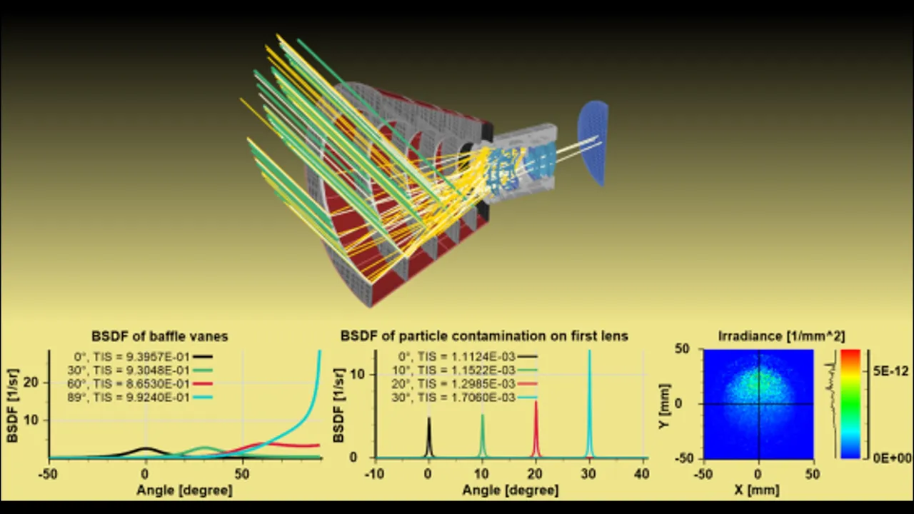
[00:37:13]There are many terms and I would like to familiarize you uh familiarize you with these terms. BSDF is the generic term for measured scattering of light and there are three specific varieties of BSDF. BRDF and notice the second letter here. R means reflection. So BRDF is reflective scatter. BTDF which is transmissive scatter. Okay. as with light as we scatter through the surface and BDDF which is the defraction distribution function. So scatter intensity or cosine corrected BSDF is a little bit different. In the old days people measured the scattering properties of a surface by measuring the scattering intensity watts per stadian normalized to the incident power watts.

[00:37:57]And this differs from the BSDF by a factor of a cosine of theta. So in other words, if someone says I'm measuring cosine corrected BSDF, you're talking about a factor of the cosine. Typical BSDFs. Well, okay, I've got a surface and it's polished. What would be my BSDF for that surface? Well, they're very shiny, so light falls off very quickly. So, we're going to have a slope of our ABG model, and that slope is going to be reduced drastically as we move off from the speckler area.

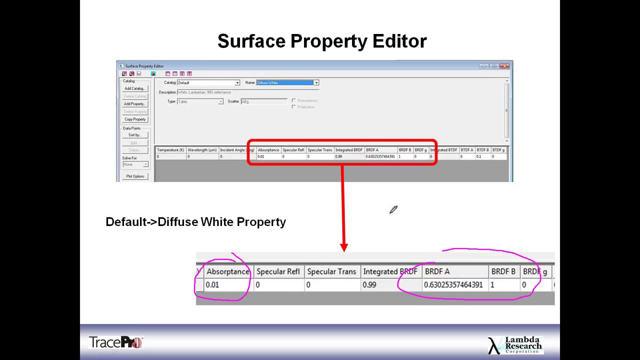
[00:38:30]Therefore, values of G from 1.5 to 3.5 for the G value on a very polished surface is very common. Well, what's the most common? A value between 2 to 3. B is small, which means that we fall off quite quickly. Uh we have very little scatter is what I should say. Uh 1 E - 6 to 1 E - 10 depending on surface statistics. Uh contamination BSDF where you have dust or something on a surface is similar form to micro roughness and you can model it as such. Diffused surfaces like blacks and things of that nature are usually lamburion. Therefore, there is no slope. Pretty much light is scattered pretty evenly across that surface and off that surface angly. So you're going to have pretty much a G or slope of zero. The BSDF is perfectly lamburian. Many baffle coatings come close to this. For instance, like chemlaz 306. If not lamburion, typically B is large.1 to one and G is large 2 3 4 56. So in other words, um you can have things like alenodide coatings, mirror 3. Mirror 3 would be a polished surface that would have a very uh a value between two and three usually with a B small. A black surface, say something like a painted black or a kryon black would have a G equal to zero if it's very very flat black and uh have a very a large B between 0.1 to one and G, you know, large as well. So here's what that model would look like. the the um the red line here is the measured surface and we fit a line to it. These values are very very small. So I have a ABG model where my A is this value over here. My B is my value over here and my G is the slope over here and G is probably is going to be a negative number but we take the absolute value. So our numbers for this would be this number here is a 0.0025 0025 B which is over here at 0001 and then finally I'm sorry G uh B over here which is 001 and G is 1.8. So there's our values A B G. Okay, that's the numbers we put into trace pro for our AG model. If we took a look at a spreadsheet and this is on our website, you can see the RMS roughness, you can see a correlation length and the wavelength and there's a nice little spreadsheet. put these values in and trace pro will automatically give you the AVG coefficients that you would put into trace pro. So you can just download this off our website. I think it's in the technical support area. And so if we take a look at a a zeroorder path or a straight shot path, this is what's happening. We have a cassagrain telescope which has a secondary mirror here, a primary with a hole in it and our detector back here with a lens in front of it. A straight shot would be a ray that goes straight through the primary hole and strike our detector. Not hitting any of our baffle surfaces or doing no scatter whatsoever. Second type of telescope surface. I've got a little hole over here. Uh here comes the light right through. Never strikes any of my surfaces or it goes through the lenses and goes and focuses on my detector. So these are straight shots. No scatter involved. We want to get rid of those.

[00:41:33]Those are our worst ones.

[00:41:35]But the big question is what can be seen by the detector? What are my critical paths? Well, to determine this, to find out what your critical objects are, those that may cause me to have stray light problems, we can trace rays backward from the image plane. And we can see which rays and which surfaces hit what what surfaces. And these are are critical objects and they are seen by the detector. So what you do is you make the detector surface into a surface source. You define the source immediately before the detector pointing backward. You display the flex report to determine which surfaces the detector sees after you do the ray trace. And you can use ray sorting to see the path of the rays and how they reach those different surfaces. In a similar way, you want to see what your hot objects are. Those are the rays that are illuminated by your sources. So you create a a once again a source that enhances your full field and you trace rays back into your system.

[00:42:32]And those those surfaces that can both be seen by the detector and illuminated by the source are your critical surfaces. And you want to make sure that if those are not your lenses and mirrors that you coat them, move them, block them, or paint them and get rid of them.

[00:42:48]So either illuminating or seeing a path should be blocked by baffles or other words mitigated by those four techniques.

[00:42:55]So once again, non-optical surfaces should not be seen by the detector if possible and they should not be illuminated as one of your hot objects.

[00:43:02]These are your critical surfaces and you want to make sure you get those out of your particular system. Finally, you can consider different paths for cases of before and after the aperture stop. So you also want to look at angular uh sets of information of how these rays are going to come off that surface towards your detector. You can see if you can put beam beam dumps in there. You want to be able to capture and block those rays if possible. You want to move that light to another area if you can. You want to coat them. If you can't do either of the first two to bring that light down as far as possible and if it is a lens or a mirror, you want to code it. And then you can use the analysis tools in Trace Pro. You can do ray sorting. You can look for a ray display to see the path of the stray light stray light. You can do a radiance mats. You can do a radiance map to see where the paths and straight hotspots are. You can use these in conjunction with each other. You can do incident rate tables, ray history tables. You can use the path sorting and analysis mode in Trace Pro 7.1. It's new. It really helps you out.

[00:44:04]If you have a large amount of rays and you want to really do a full analysis, you may want to go into simulation mode.

[00:44:09]And we have ray path sorting to a file in that case so you don't run out of memory. So pretty much you can also use ray storing for display. Here's where you see it. You use the analysis ray sorting. You can select different source types. You can select the number of rays you want to see. And as we see here, we have incoming rays that bounce around inside of our baffle. And then the important sample rays get to our detector. So we can see how much light actually is caused by stray light in this um simple Newtonian telescope. You can do ray sorting for ray type. If you say I want to look at multiple scatter, you can bring this particular window up, do the multiple scatter and then only see the contribution from that multiple scatter.

[00:44:51]You see sorted on multiple scatter arrays down here in the bottom right hand corner of the radiance map showing us only the light that gets here for that particular selected path. So you can use them in conjunction with each other. Ray sorting with a radiance map.

[00:45:04]Ray sorting for hotspots. You can display the selected rays that are contributed by this particular ray path over here. In fact, you can hold the left mouse button down, draw a rectangle, and then say, I only want to see these rays for this contribution in my ray sorting, and it'll show you only those rays in your race sorting in your system view. So, there we go. We're sorted on multiple scatter arrays. We create a little rectangle. We then choose display selected rays over here and it shows me only those rays in my system view.

[00:45:39]That's how the process works. Now if you want to take a look at a particular ray, you can do that as well. You can do the incident rate table which shows you every single ray that's incident on the the image plane in this case because I've selected that in the system tree. I can then select the ray, go into analysis and say display selected ray. It will show me only that ray path for that particular path. And you can go down for each one of these and select them and trace will automatically update the system view for just that selected ray. So once again, incident ray table works for the visualization of the ray.

[00:46:12]Coincidentally, the ray history table works the same way. We can bring the ray history table up. We're looking at ray number two. We can ask that once again to analysis display just that ray. And it will do that. So we can see that. And the ray history table shows us the complete history of how the ray got through the surface. We can see how it bounced off the different surfaces, how much power it had, and what positions it actually hit. So, we can then visualize how a stray p stray light path occurred.

[00:46:39]And now we have a mechanism to get rid of it. Finally, ray path sorting. This is done in simulation mode. You can see the ray path. It'll tell you how the ray got there. It will break down the flux just like it did in analysis mode, but this is if you're tracing lots and lots of rays. And this is done in the ray trace options in the simulation output where we say collect exit surface data. We then specify that we want to save our ray data to disk, our rate history to disk and sort our rate pass. This is the one right here. This option is the one that creates our rate pass sorting file.

[00:47:13]Okay, that's all I have for you right now. I'm going to open up the webinar for questions. I'm sure you have quite a few. And uh our Andy Knight, our organizer, is going to come back and uh help us out here. Does anyone have any questions?

[00:47:28]Thanks, Mike. Nice job. So, yeah, we are looking at the question window here and there is nothing so far. Guess you did just an excellent job and everybody understands everything.

[00:47:42]Well, I hope so. Did anyone have any questions on important sampling or any of the methods or the any of the analysis techniques that we used here or how a specific system could be analyzed?

[00:48:03]Well, this webinar is going to be placed up on the website so you can go and look at it at your leisure and you know you can download these slides. You can download and listen to the webinar. Once again, hope I didn't go too fast for a lot of people out there. If you have specific questions, don't hesitate to uh to send an email out to us and I'll be glad to explain anything that uh we've gone over. We've got a couple popping up here, Michael. So, I have one here. Um, thanks for explaining important sampling. Is there a recipe style tutorial available that walks through important sampling setup and usage?

[00:48:40]I believe there's a tutorial on the website there. There is one, Mike. Uh this is Dave for uh uh autoimp important sampling using the uh I believe the cook triplet lens. So that's under the tutorial section on the website. That is correct. Thanks. Okay, great. Uh next qu question. Can you choose array directly from the display rather than from the table of ray paths?

[00:49:08]Uh no, you can only select them from the path sorting uh table, from the instant ray table and from the ray history tables. You can't uh point you can't click on the thing and it will then show up and uh show you that particular path for that particular ray at this time.

[00:49:25]Will the polarization map be updated with ray 41?

[00:49:31]Um that's a that would be a feature request. I will be glad to add that to the feature request and no currently no you cannot um have the polarization map uh be updated with race ordering.

[00:49:44]Okay, I'll put one more. Oh, here we go.

[00:49:46]Got another one. How do I know what threshold to set? That is a very good question. Um, if we bring up Trace Bro. Now, let's bring up that demo triplet and we rate trace a system. If you go into the rate trace options, you can see what your threshold is set to. If you don't if for a u a transmissive type system like this, the flex threshold is set to 0. Z1. If you don't see any rays making it to your detector, you haven't traced an uh you haven't set the flux threshold low enough. But there's a special report called the flux report. And the flux report has many many different table entries. And you're going to see things like lost escaped model loss flux threshold. If these values are large compared to the flux you have coming in, you know that your flux threshold is not set low enough. So you need to change your flux threshold to these values are low in retrospect to what your incident rays are on that surface and they are you can see here that I've got 296.719 watts on the first lens surface and the lot the flux threshold is lost I'd say 253 that's such a small percent that's a really low threshold my threshold set correctly if this is a very large number you need to go back go to your view options and I'm sorry. Go to ray trace options right here and set that flux threshold lower.

[00:51:27]You see right now it's set to 0.001. Now what happens if I set this lower? Oh, actually let's go one more. What's going to happen is the rate traces are going to take a lot longer.

[00:51:38]The whole screen is going to turn blue.

[00:51:40]And if I go back into my flux threshold, you can see this value is much much smaller now. So I trace more rays. it was within a valid time. I really didn't change the amount of power very much incident on it. But now I'm not only getting sec I'm not only getting first order ghosting I'm getting second order ghosting. And what happens is that if I ask for a ghost image analysis by using my pass sort table I have to select a surface first by the way. Let me just grab this my detector surface over here. So that's what you have to do. Then you can see all the different paths. So these are my second and fourth order paths. And you can see my instant flux getting much much much smaller down here for those those four bounces in my ghost. Now if I go back and set this ray trace report and I set this back to 0001 and reray trace, you see my pass get much smaller.

[00:52:40]I'm no longer getting those ghosts. And am I really losing or changing my first value, which is my spectre, which is 99.45% of all the power that gets there.

[00:52:50]So, it depends on how far you want to go. If you want to see your second order goes, you're going to have to drop your flux threshold. But how much is enough, that's up to you what you want to look for. I think I've answered that one.

[00:53:04]So, I'll put one more uh request for questions out there before we wrap up.

[00:53:12]Looks like everybody's satisfied, Mike.

[00:53:15]Well, great. I'm glad that you um joined us and uh we'll have another one next month. And uh if you have any ideas of what you'd like to see in terms of a u a webinar, please send your uh send email to saleslamarez.com and we'll try to get that up for you.

[00:53:32]I wish you all a great day.

[00:53:34]Okay. And thanks again everybody. Have a great day.

[00:53:42]We will post a link on the homepage for the slides as well as where to download from the webinar and that'll be up a little bit later today as we uh create the recording. Have a good day everyone. Bye for now.