




![[Latest Version] ELISA (Sandwich Method) Procedure – Enzyme Linked Immunosorbent Assay, Elabscience](https://i.ytimg.com/vi/_lbe7D1sRL8/maxresdefault.jpg)






![[Wikipedia] Strictly standardized mean difference](https://i.ytimg.com/vi/G5wu6m1iKU8/maxresdefault.jpg)








This video demonstrates how to perform fluorescence intensity measurements using the Tecan Spark microplate reader and SparkControl Software, covering key principles including plate selection (clear plates for homogeneous solutions, black plates for fluorescence, black-walled plates with clear bottoms for adherent cells), excitation and emission wavelength selection with the minimum distance rule to prevent crosstalk, gain optimization (optimal, calculate from well, extended dynamic range, manual), Z-position optimization for focusing, settle time for liquid stability, and multiple reads per well for spatial averaging, all of which collectively ensure accurate and reproducible fluorescence data collection.
Fluorescence Intensity Measurement: Tecan Spark Microplate Reader Tutorial
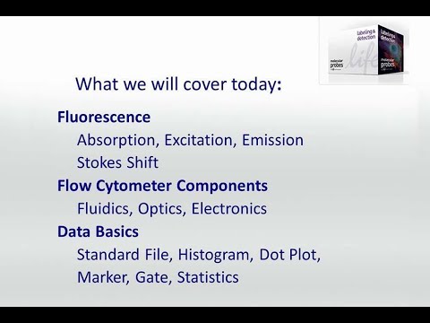
Added:Fundamental principles of fluorescence, including fluorophores, excitation and emission spectra, and the Stokes shift.
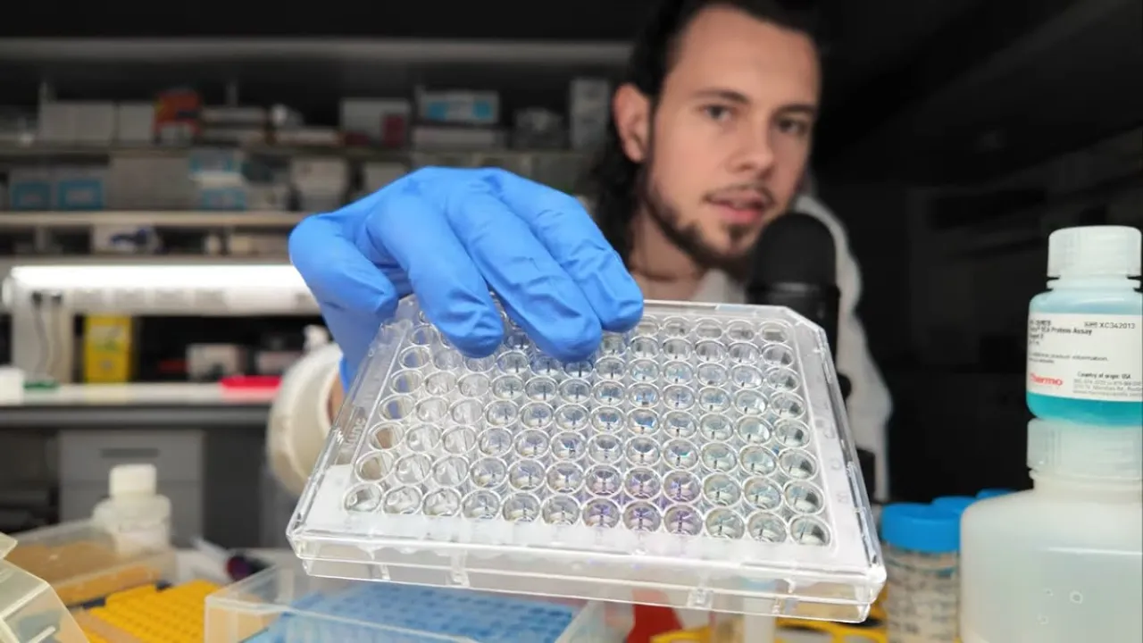
Basic understanding of microplate assay formats (such as 96-well or 384-well plates) and standard liquid handling practices.
General concepts of optical detection, including how light sources, monochromators, optical filters, and photomultiplier tubes (PMTs) function.
The concept of signal-to-noise ratio, background fluorescence, and the role of positive and negative controls in quantitative assays.
Advanced fluorescence-based techniques such as Time-Resolved Fluorescence (TRF), Fluorescence Resonance Energy Transfer (FRET), and Fluorescence Polarization (FP).
Quantitative data analysis workflows, including curve fitting, statistical validation, and calculating limits of detection (LOD).
Troubleshooting common experimental artifacts such as photobleaching, chemical quenching, autofluorescence, and the inner filter effect.
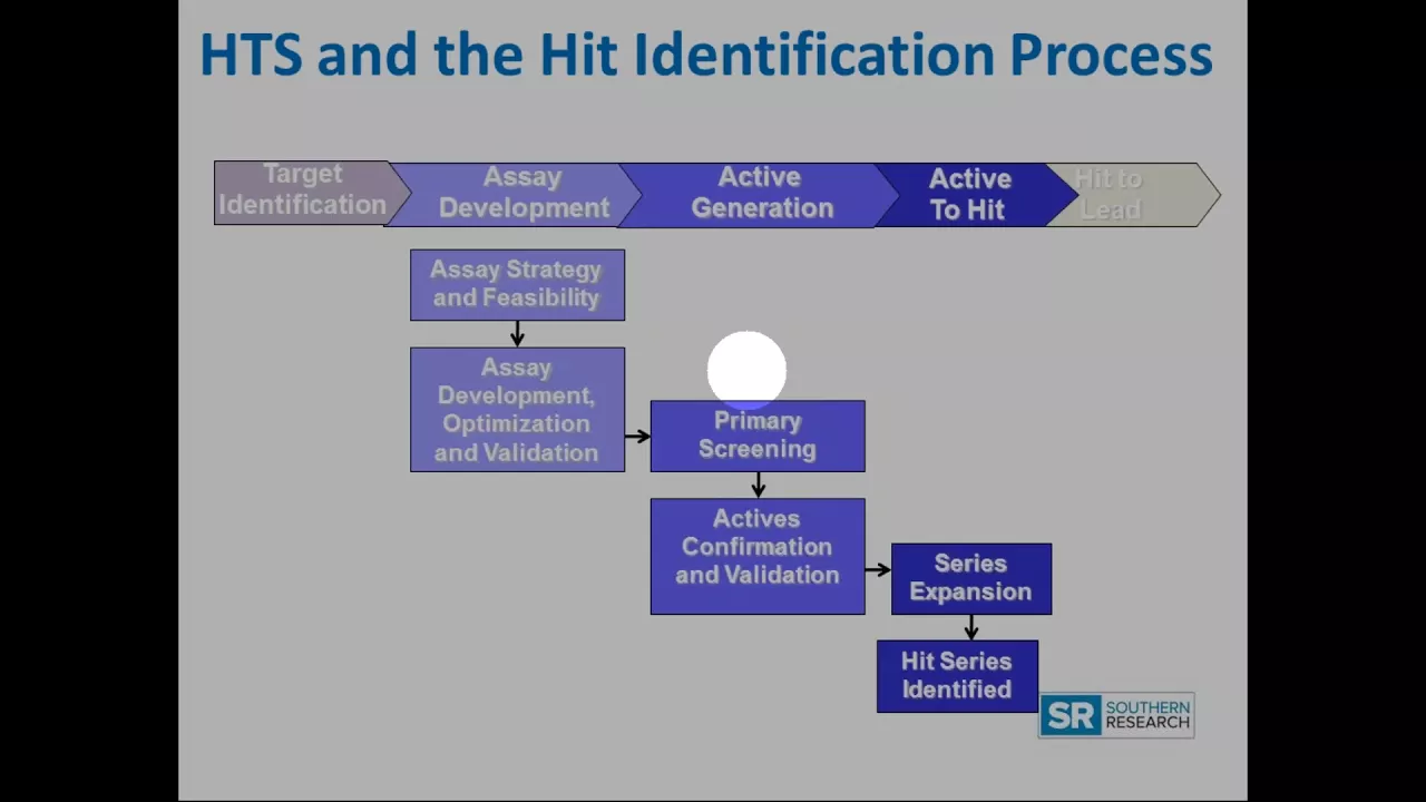
Integration of microplate reader protocols into automated high-throughput screening (HTS) workflows and robotic liquid handling systems.
18.2K views193likes22:46Original Release: 2019-10-13
hi this is an overview of how to take fluorescence intensity measurements with the T can spark microplate reader and spark control software with your reader and computer turned on and the status light of the reader at magenta launched the spark controlled dashboard software and once in the dashboard you'll click on the method editor new button to begin writing a method the first step in the creation of any method is to select a plate definition to match the plate you're using I want to first explain though that I'm using these fluorescent highlighter pens on this clear micro plate where the Pens have been drawn across the bottom to create some signal if you're ever in a pinch for a fluorescent standard or something to at least test the functioning of your instrument then pens like these are very useful so in this example we're going to select a clear flat transparent micro plate and for this video you cannot see the drop-down list here but if you could it would look a little bit like this where you could scroll up and down and select from a variety of different plates and if you don't find the plate that you're looking for you would contact he can and they could help provide you with the correct definition it's worth noting that if you're measuring solutions of fluorescence that an all-black plate is the best way to go whereas if you're measuring adherent cells where you have a lid on the plate then a black wall plate with a clear bottom is best again for our example we're using a clear plate and here we're going to click and drag across the wells you want to measure and then click and drag and drop the fluorescence intensity strip into the screen you don't have to put a name here but I'm going to type in yellow pen just as a way to reference the reading and then the decision is whether to read from a top for homogenous solutions of fluorescence or if there are here it's cells then we can read from the bottom even though there's marking pen on the bottom of this plate and it might make sense to read there I am going to read from a top to demonstrate some other features the next step will be to select our excitation and emission wavelengths and depending on the instrument you have it may be equipped with filters or tunable wavelength monochromators or even a combination of both called fusion in this case I've got a fusion instrument so I have both selection of filters and monochromators and just for the sake of showing you the filters they are loaded on what's called filter slides through the front of the instrument each filter slide for excitation and emission holds six filters and users can customize these slides holders with different filters as they see necessary the filters have fixed bandwidth of course but the monochromator mechanism on the spark can be either a fixed bandwidth system if you have a standard spark or it can have variable bandwidth if it is a enhanced fluorescent spark and the enhanced model has adjustable bandwidth from five to fifty and while you can't see it in this display here if you click on these fields you can select different bandwidths to be used during measurements when entering your wavelength and bandwidth settings it's important to understand the minimum distance rule the minimum distance is the distance that must exist between excitation and emission wavelength settings in order to prevent what's called spectral overlap it's also known as crosstalk and crosstalk can result in high background during a readings that looks like fluorescence when it's not here's an example where the wavelength settings are correct and there's low background along with some good signal but here's what happens if the wavelength settings in this case where the emission is too close to the excitation where you get much higher background in the readings and this may look like fluorescence but it's actually bleed through where the excitation light is striking a sample and being collected back up through the emission optics where it registers as signal when in fact it's just scattered light arriving at the detector from the excitation channel to determine the minimum distance of your settings take the bandwidth of excitation plus bandwidth of emission plus five nanometers and then take the emission wavelength minus the excitation wavelength and that difference must be greater than or equal to the minimum distance in order to avoid cross if we evaluate our current settings the sum of the bandwidth as plus five nanometers gives us 45 nanometers as our minimum distance and what the current wavelength settings 535 minus 485 gives us 50 nanometers and 50 nanometers is greater than 45 so we have not violated the minimum distance rule and we can take readings without cross talk another way to visualize how minimum distance plays in to the correct settings is to go to this fluorophore list and in this instance I'm gonna pick fluorescein you can't see the pulldown here but I'll bring up a screenshot to show you what it looks like but once you have picked fluorescein or some other dye it will show you as in this case the in blue the spectral excitation profile of the dye and in red you'll see the emission profile and then depending on your excitation and emission wavelength settings as well as your bandwidth you can see these vertical lines here for the excitation those represent the wavelengths that will be passed through to the sample for excitation and over here the red vertical lines represent the emission wavelengths that will be collected and passed on to the detector and you can click and drag these around to in this case increase the emission or decrease it and once I violate the minimum distance rule here which happens to be because of the bandwidth being 20 and 20 plus 5 that's 45 once I get closer than 45 you'll get a little warning here indicating that this would result in a crosstalk detection and so ways to sort of overcome this would be to obviously move the wavelengths apart but if the dye was such that you wanted to be very close in terms of excitation and emission you could adjust the bandwidth if you have an enhanced spark so I could potentially do that reduce it to 10 now this lets me get closer to parking things over the emission alternatively I could reduce the bandwidth on the excitation as I'm doing this of course I'm letting less light into the sample and collecting less light back which could result in some lower sensitivity but this is something that you just have to experiment with but by having narrower bandwidth you can obviously have a smaller minimum distance between excitation and emission I'm going to go ahead and back things out to our twenty and twenty again and get our emission back up to a healthy minimum distance here and now we can cover some other topics the next step will be to click and reveal the advanced settings for flashes the default number of flashes per well is 30 and this is intended to give you the most ideal results for most general purpose fluorescence readings there are instances where you can use one flash to go very quickly but with risk of there not being as much consistency as you may want adding more flashes like three five ten flashes will give you more averages per well and improve the consistency of the data while still maintaining some read speed you can play around with different read or flash settings but for now in this example I'm going to stick with about five and I generally stay between five and ten for most applications for the gain setting this is how the instrument adjusts the voltage on the detector to affect how much signal is presented in the data output and the signal range is zero to 65,000 so when you select optimal this is where you do not know where the brightest sample is on the plate and you'd like the reader to go and find that sample and adjust the voltage so that that samples are a few value is effectively forty-five to fifty thousand counts once it finds the correct gain to generate that value it will read the entire plate at the gain it finds this way you do not run the risk of any well on the plate having what's called an over value where it goes beyond the range of 65,000 there is an additional option for determining gain and that is called calculate from well you would use this feature if you happen to know where the brightest well is on the plate this saves the reader time of not having to go around and find the bright well on its own so this is a little bit faster way of measuring again it would go to the well you designate it would adjust the voltage so that that sample would have a count's between 45 to about 50,000 you won't be able to see it here but there is a pulldown menu visible on my screen that's not showing up in the video but you can click on the pulldown menu and select the wells that you want it to go to do this calculation from there is a third means of determining gains and it's called extended dynamic range this is a way for the reader to use two separate gains to measure the samples and by virtue of this it can give you a much broader range of signal intensities from 0 to 6.5 million you would use this feature if you know that you've got very very weak samples in your plate mixed in with some very very bright samples and you simply just give this a try and see what it gives you but it is a way of being able to get more range out of the instrument than you otherwise could by just measuring at one gain lastly there is a way of simply fixing the gain manually between a value of 0 to 250 where of course as you go from a small gain value to a large one you will increase the amplification of the signal and you will find many cases where you've read the same assay many times and by choosing optimal gain or calculate from well you will see a very similar gain appearing for that assay and therefore you can come here and to simply type in what that game would be so you're not always having to reoptimize each time be mindful that ideal gains for instruments like the spark will range between about sixty and a hundred and eighty so you'll see that for very very bright samples the instrument depending on its settings may try to use a very low gain something under sixty or four samples that are very very dim and and maybe there is no fluorescence it may come back and give you a game that's much beyond 180 and the instrument can at very high gains produce what appears to be signal when in fact it's just amplification of noise so again just it's best to try to operate within a range of about 60 to 180 if you can also on the spark standard model you will see that there's a choice of a 50% mirror and a 5/10 dichroic mirror if you need an examination of what dichroic mirrors are please consult your teak and manual or perhaps other videos that will be produced on this topic but for now just know that the standard models got a 50% and a 5/10 whereas the model like this one with a enhanced fluorescence optics has a choice of additional Mayor's plus one user-defined mirror that you can insert and use to address other wavelengths within the range of the spectrum for purposes of this example I'm going to leave it as automatic and let the reader decide which mirror to use for the wavelength settings that have been selected also the spark can move the plate carrier up and down in the Z direction much like a microscope stage in order to focus at the right depth within a well if you set this to automatic or calculate from well and designate a well that you know to have some fluorescence in it such as again perhaps sending it to f1 it doesn't have to be the well with the brightest sample but certainly a well where you know there is definitely some representative fluorescence in that well then the instrument will move the play carrier up and down identify the depth at which it gets the best say and then it will read the entire plate at that depth it will also report this Z position and both the gain values its determining here in the data output so you can use those values again should you want to repeat the reading and not have to go through the exercise of making the reader determine these values a second time despite that it's going to find the same values on the second reading again there's a parameter here called settle time this was addressed in the absorbance video but essentially if you are using 96-well plates and you are going to fill them with more than a hundred microliters you can leave the settle time as zero if you fill the wells with less than 100 microliters there's a risk that some of the liquid on the surface of the well will vibrate as the plates being moved and that vibration can be detected once the flashes are applied so for 96-well plates if you're going to use less than 100 you can enter values here between 100 and 500 milliseconds as a sort of a way of ensuring that this vibration goes away also if you're going to use larger volume wells like something between a 48 well plate in a 6-well plate then certainly some amount of settle time is necessary here because as those plates are moved some of that solution begins to move around and you don't want the solution still moving at the point in which readings are taken so for those again you may need to go as high as a seconds worth of settle time in order to get the best results for this example today of course there is no volume in the plate I don't even have to worry about it'll settle time so I'm going to leave it at 0 there's a more advanced feature with the software called multiple reads per well if you were to look at this it's sort of obvious that it's going to take additional readings at different physical points inside the well based on the number of flashes you've given it so if I've got five here it would flash 5 here 5 there and so forth and give me individual fluorescent intensity values for these 5 points plus an average of those and standard deviation for them depending on the pattern that's picked and you can get pretty carried away with different types of patterns and densities here getting some averages from the wells if there are features in the well that you feel must be measured independently so that's how that feature works you can also consult your manual or your T Ken representative for more help with this topic for this example we'll turn off the multiple reads per well and just use the center default read of five flashes per well in the center of each well we will also drag and place a move plate out step into the protocol and then this example will also go back to having optimal gain as the setting and calculate Z from well f1 and with that we can go up here and press Start and collect our measurement the instrument will first go to well f1 and determine the optimal z distance at which to focus and we'll use that distance for measuring all the wells we'll also optimize the gain by finding the brightest well setting the gain to make sure that well has 45 to 50 thousand RFU and it will use that gain to read all the wells in the plate so you'd be able to tell if the instruments doing things correctly if you can see counts on your plate between let's say upwards of forty five to fifty thousand and you can also see very small less intense samples that might be representative of blanks in the example here the orange highlighter pen and the top has some fluorescence when excited at forty five and five thirty five whereas if we go back to our display here we can see that pink highlighter pen does not excite an emit in this range whereas the yellow highlighter pen does have excitation and emission that's pretty decent in the four eighty five five thirty five range may also view the data as a color heat map again it's the pink highlighter pen that's giving the most fluorescence here the excuse me the orange and then the pink is very dim and the green or yellow highlighter pen not so much but still more so than the pink highlighter pen all right so we got an export to excel as well see if we can find that file it is this one here we can see that the gain of picked was seventy three so it's above sixty so that's good it's showing us that it used the dichroic mirror the 510 that makes sense because a 510 mirror would be able to split the light between 45 and 535 the z-position reported is here at 16,000 804 so you could if you wanted to read these plates again or this plate again go back and fix the gain manually at 73 and the z-position at 16,000 804 and you'd be good to go here's the data we can see that we've got values upwards of about 52,000 here and again some some weaker looking signals here and this is a good example of how there's a nice spread of signals between low and high now that we have some data where we've got ideal gain an ideal Zee let's go and change things so that we can see how these different settings like bandwidth and wavelength and gain affect the signal so our previous ideal gain here for this plate was 73 we're going to change the gain to 83 and we'll fix the Z at the previously determined optimal Z and run this again so now you'll see that once we've raised the voltage on the detector by a factor or by 10 let's say then we're getting over values which means it's over 65,000 and it's also increased the intensities of other samples on the plate so what's going on here is that for every change of the gain by about 10 you will see an approximate 1.8 to 2 times change in the intensity another strategy for changing the intensities of your samples while holding other things like the gain or wavelengths the same would be to alter the bandwidth increasing bandwidth distance makes more light and and more signal and decreasing the bandwidth would decrease the signal in this example I'll go ahead and change both band widths to 10 so we should see less signal and we'll go ahead and read that and see what happens and comparing this data to the previous data you can see that the signals are now considerably smaller now while keeping the gain and the Z position the same I'll change the bandwidth spec to 20 but then we'll switch the excitation wavelength is something that's more ideal for the orange highlighter pen and the yellow highlighter pen a wavelength like 450 would work well here and we'll see what sort of result this has when we measure it again the excitation of 450 is now driving all of the signals for the orange highlighter pen in a and B off scale but in turn it's also a more ideal excitation for the yellow highlighter pen as you can see here by these increased signals for the orange highlighter pen in rows a and B a strategy for lowering the intensity there to something more acceptable would be to reduce the bandwidth on excitation and or emission to lower the gain or to move the excitation or the emission wavelengths maybe even both to something better less ideal once you've arrived at some settings that you'd like to keep as a method you can go up here to file and choose save as and while you can't see it on my screen I'm clicking save as you can enter a name for the method I'm just going to name it something like test method version 1 and then when you hit save the software will populate the dashboard with a tile you can see it here called test method version 1 if you were to click this it will bring up the method to run you can open this part here and see which Wells will be measured and when you press Start that will go right into reading now this is a simulation so everything's happening quite quickly it's not actually driving an actual reader in this example but you can see that you get your data here and then your export to excel this concludes the video I hope you've learned something useful and thank you very much for watching you
Up Next

40:34
The Theatre of the Absurd: Martin Esslin's 1960 Analysis
@ATheoryReader
838 views•2024-05-01

12:54
Triumph of Orthodoxy Icon: Byzantine Art & History Explained
@BenCallan
2.1K views•2024-08-06

9:49
FastAPI vs Flask vs Django: Choosing the Right Python Web Framework
@TechWithTim
302.5K views•2024-05-26

1:42
Game of Thrones Opening Credits: A Cinematic Analysis
@gameofthrones
46.3M views•2011-04-18
Related Study Plans & Knowledge Roadmaps
Structured learning paths in General & Interdisciplinary Studies
general-studies
Elevator Engineering: History, Physics & Cities
01From Hoists to Safety Brakes: The Dawn of Vertical Lift
02Hydraulic vs. Traction: The Engineering Physics of Elevators
03Modern Speed, Safety, and Algorithms
+ 2 more learning modules
12h5 modules
Explore Roadmap
general-studies
Rubber: Material Science, History & Geopolitics
01Origins of Natural Rubber & Mesoamerican History
02The Chemistry of Natural Rubber & Vulcanization
03The Geopolitics of the Rubber Boom & Colonization
+ 2 more learning modules
12h5 modules
Explore Roadmap
general-studies
Containerization: Evolution, Logistics & Trade
01Ancient Trade & Bulk Cargo: Amphorae to Barrels
02The Industrial Revolution & Cardboard Packaging
03The Containerization Revolution: Malcom McLean
+ 2 more learning modules
12h5 modules
Explore Roadmap
general-studies
Textile Tech: Evolution, Labor & Global Impact
01Pre-Industrial Textiles: Handloom & Cottage Industry
02Mechanization: The Spinning Jenny to the Power Loom
03The Factory System & Global Labor Transformation
+ 2 more learning modules
10h5 modules
Explore Roadmap