This video demonstrates the practical assembly of a micromouse robot, covering key electronics skills including SMD and through-hole soldering techniques for PCB assembly, motor mount installation for drivetrain components, and encoder integration for movement tracking. The creator explains how to systematically build and test robot peripherals, addressing common bugs encountered during the process. The project showcases fundamental robotics concepts such as using resistors and capacitors for power regulation, implementing motor control systems, and incorporating sensors for navigation. This hands-on approach illustrates the iterative nature of robotics development, where testing each component individually before system integration ensures reliable performance.
Micromouse Build: Soldering, Drivetrain & Encoders for Maze Solving
Added:Fundamentals of Soldering: Familiarity with basic hand-soldering safety, tools (flux, solder wick), and the practical distinctions between through-hole and Surface Mount Device (SMD) components.
Successful soldering begins with understanding materials and preparation. Two main solder types exist: leaded solder (easier for beginners due to lower melting temperature) and lead-free solder (requires higher temperatures). Solder diameters vary for different applications—thicker for large wires, thinner for small components. Critical preparation includes cleaning metal surfaces with isopropyl alcohol (91%+ concentration) to remove dirt and oxidation. Flux application is essential despite solder containing internal flux, as it cleans and guides solder flow. Ventilation is crucial for safety when working with solder fumes.

Solder is an alloy of tin and lead with a melting point nearly 100° lower than either pure metal. This unique property allows soldering without melting base materials. Wetting action occurs when molten solder flows over heated metal, dissolving and penetrating the surface at the molecular level to create permanent bonds. However, oxidation forms when metal contacts air, creating a non-metallic film that prevents proper bonding. Fluxes derived from natural rosin dissolve and remove these oxides, enabling successful solder joints.
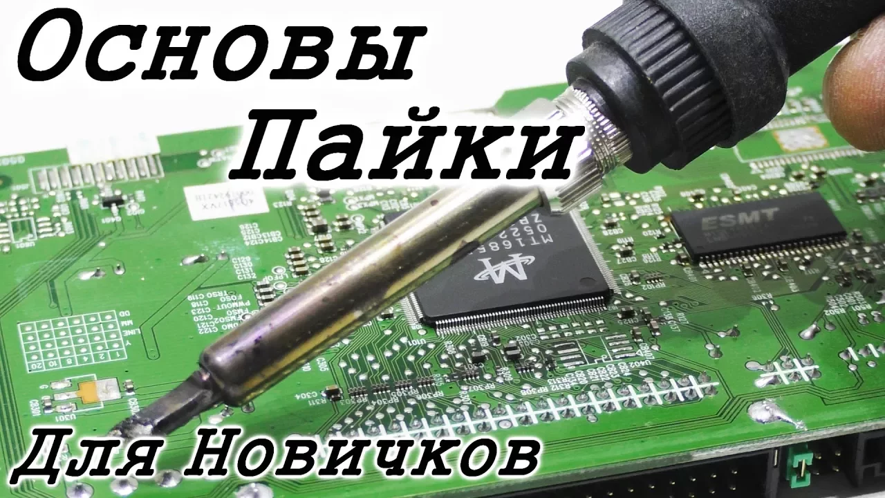
This video teaches the essential fundamentals of soldering for beginners, covering the selection of appropriate soldering tools (Soviet soldering irons with copper tips are recommended for newcomers due to their low cost and ease of use), essential materials like solder (ПОС-61 and CAD-3), flux, and soldering acid, and practical techniques including tinning the soldering iron tip, preparing wires by stripping insulation and twisting strands, soldering wires together, tinning circuit board traces, soldering connectors like tulip connectors, soldering LED strips with proper insulation using heat shrink tubing or thermal adhesive, and using a heat gun for delicate components like microcircuits.
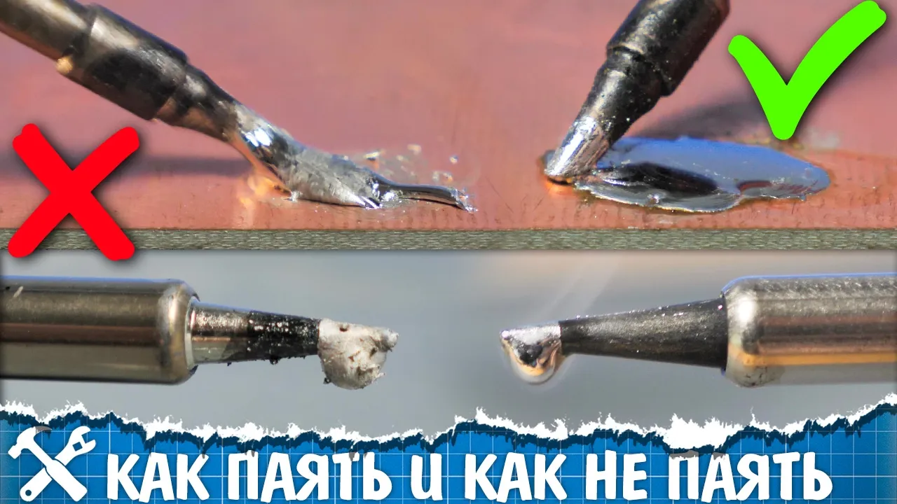
Soldering is a technique for joining metals using a low-melting-point alloy (solder) that flows between surfaces when heated, creating a reversible connection unlike welding; the process requires proper equipment including a soldering iron (with options ranging from basic nichrome models to advanced temperature-controlled units), solder with flux core, and appropriate flux (such as rosin, LTI-120, or gel fluxes for SMD components), with optimal temperature around 270°C and successful joints requiring proper wetting where the solder spreads smoothly across the metal surface.

This comprehensive section covers the essential fundamentals of soldering. It begins with the necessary tools: soldering iron with stand, solder in coil, flux with brush, wires, and motor. The process starts with preparing the soldering iron by cleaning the tip with a wet sponge and applying flux (rosin in alcohol solution). The tip is then coated with solder to create a shiny, receptive surface. Wire preparation involves stripping insulation using specialized tools or wire cutters, then twisting wire ends neatly before soldering. Each wire end must be pre-tinned with solder to ensure reliable connections, as solder alone provides weak mechanical holding power. This preparation phase is critical for successful soldering outcomes.
Basic DC Motor Physics: Understanding how brushed DC motors operate, including the relationship between voltage, speed, torque, and gear ratios in mechanical drivetrains.

A DC motor consists of the same basic components as a DC generator: a coil (armature), a magnetic field, a commutator, and carbon brushes. However, in a motor, current is supplied from an external voltage source (like a battery) through the commutator to the coil, causing it to rotate. The commutator reverses the current direction in the coil every half rotation, ensuring continuous rotation. The current-carrying coil experiences a force in the magnetic field that produces torque, which causes the coil to rotate. This torque is the rotational equivalent of force and drives the mechanical motion of the motor.

A basic DC motor consists of four main components: a pair of magnetic poles, an armature made of a single turn loop, a commutator, and a brush assembly. With voltage applied, the right conductor is pushed down while the left one is pushed up. Adding another loop and two commutator segments ensures motion at all times since one commutator segment always contacts the brushes while another moves away. More loops result in smoother motor motion.

A basic DC motor consists of an axle with a wire loop wrapped around it, connected to two commutators (copper contact points) on each side. The axle is non-conductive while the commutators are conductive, allowing current to pass through them. Stationary brushes maintain electrical contact with the rotating commutators. When current flows through the wire in a magnetic field, the left-hand rule determines the direction of force on opposite sides of the wire, causing the axle to rotate continuously.
![How does a DC motor start running? [EN]](https://i.ytimg.com/vi/9_bC6USqUOQ/maxresdefault.jpg)
DC motors operate based on two fundamental physics principles: magnetic flux and Lorentz force. Magnetic flux (Φ) measures magnetic field lines passing through a coil, calculated as Φ = B × A × cos(α), where B is magnetic field strength, A is coil area, and α is the angle between field lines and the coil's perpendicular axis. When current flows through a conductor in a magnetic field, Lorentz force is generated, with direction determined by the right-hand rule (FBI rule). In a DC motor, current-carrying windings placed in a magnetic field experience Lorentz forces in opposite directions on different parts of the winding, creating torque that causes rotation. This torque is calculated as τ = F × L, where F is the Lorentz force and L is the distance from the rotation axis.
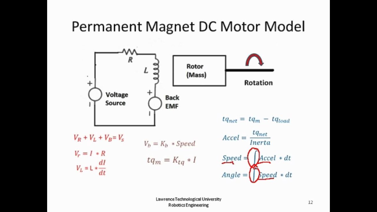
A DC motor operates through the interaction of electrical and mechanical systems. Internally, the rotor contains coils with resistance (R) and inductance (L). When voltage is applied, current flows through these coils, generating torque proportional to current (τ = Kt × I). Simultaneously, rotation generates back EMF proportional to speed (VB = Ke × ω), which opposes the applied voltage. Kirchhoff's voltage law governs the electrical side: VS = VR + VL + VB, where VR = I×R and VL = L×di/dt. Newton's law applies mechanically: τ_net = J×α, where net torque equals moment of inertia times angular acceleration. These coupled equations form the foundation for modeling motor behavior.
Rotary Encoder Principles: Conceptual knowledge of how optical or magnetic quadrature encoders generate pulse trains to measure rotational velocity and direction.

Rotary encoders use Gray code to encode rotational position. When rotated, they produce distinct LED sequences for clockwise and counterclockwise motion. The critical feature is that only one pin changes state between consecutive steps, preventing multi-step errors from contact bounce. The internal structure includes a knob, contact wheel with conducting/insulating sections, and a base with sliding contacts and dome switch. The copper spring creates tactile detents providing position feedback. This design makes rotary encoders reliable for position sensing in devices like radios, power supplies, and mice.
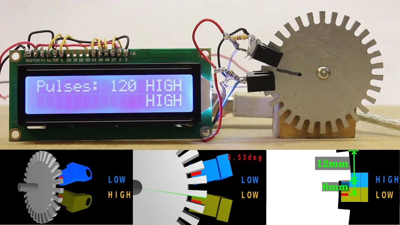
In rotary encoders, the arrangement of sensors relative to the tooth/gap pattern determines the output signal sequence and resolution; when sensors are positioned such that one tooth covers both simultaneously, the rotation is divided into unequal steps, but when sensors are spaced by an integer multiple of tooth/gap widths plus or minus half a tooth width, equal steps can be achieved, with the sensor distance typically expressed in degrees rather than millimeters.

The hosts engage in a detailed technical discussion about rotary encoder design in electronic devices. They distinguish between endless encoders (which spin indefinitely) and stepped encoders (with fixed positions and clicks). The hosts argue that stepped encoders provide superior physical feedback because users can feel when they've reached specific positions, preventing confusion. They discuss how endless encoders can cause issues when users spin beyond intended ranges, as there's no physical stop. The hosts also debate whether faders are superior to knobs for certain applications, and how the lack of physical feedback in endless encoders creates a 'one-way conversation' between user and device.

A rotary encoder contains a round pad with a conductive metal pattern and non-conductive material. Two metal pins (Clock and Data or pins A and B) sweep across this pattern. When power is applied and the encoder is spun, one pin touches the metal first, completing the circuit and being pulled low to GND, before the other pin does the same. After connections are interrupted, pins return to supply voltage. This creates voltage pulses where the order of signals (which pin triggers first) indicates rotation direction - clockwise shows B before A, while counterclockwise shows A before B. Optical encoders work similarly using light sensors through a patterned disc.
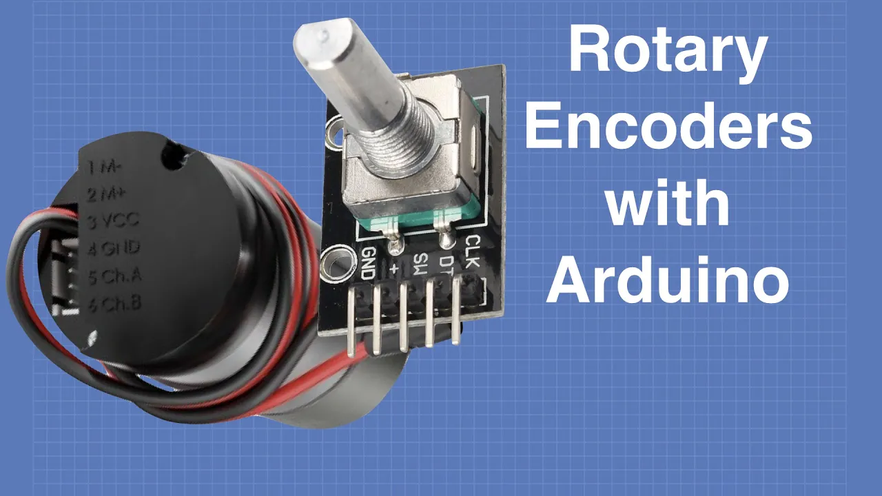
Rotary encoders are devices that measure angular rotation by generating two out-of-phase pulse signals (Channel A and Channel B), which allow microcontrollers like Arduino to determine both the degree of rotation and its direction; these encoders can be implemented as precision controls for devices like servo motors or as feedback sensors to measure motor speed by counting pulses over time intervals.
Introductory Circuit Schematics: Ability to read schematic diagrams and identify basic electronic components such as resistors, capacitors, and microcontrollers on a Printed Circuit Board (PCB).

This video teaches how to read electronic circuit schematics by identifying key components including power supply symbols (9V-15V), capacitors (104 = 100nF ceramic), integrated circuits (AM324), resistors (10kΩ, 47kΩ), photoresistors (LDR), transistors (NPN/PNP types), diodes, DC motors, transformers, and switches, along with practical assembly methods using breadboards and PCBs.

Full schematics show detailed circuit connections including component values and signal paths. Understanding schematics requires learning to trace signal paths and identify component functions. Key skills include: identifying component names and locations, tracing voltage lines through components, recognizing bidirectional data communication, and understanding how signals change names as they pass through protection circuits. The schematic serves as both a design document and a parts list, providing actual component values rather than just manufacturer names.

In circuit schematics, components connected to ground are in parallel, meaning they share a common ground connection and can be bypassed without breaking the circuit; components in series are positioned along a single line between two points, and removing any series component breaks the entire circuit path, making them essential for the circuit's function and not interchangeable with simple bridges.

Electrical circuits are represented using standardized symbols: generator (battery symbol), voltmeter (V with circle), ammeter (A with circle), and lamps (bulb symbol). An ammeter measures current intensity and must be connected in series. A voltmeter measures voltage across a component and must be connected in parallel. The direction of current flows from the positive terminal of the generator through the components to the negative terminal.

The horizontal circuit in a television has two primary functions: moving the electron beam horizontally across the screen (horizontal scanning) and producing high voltage for the tube; it consists of key components including the flyback transformer (with internal diodes forming a voltage multiplier and potentiometers for focus and screen), the horizontal output transistor, the driver transformer, the pre-horizontal transistor, and the horizontal oscillator within the One Ship chip, which also contains the microcontroller and general processor for the television.
Prerequisite Knowledge
- Concept 01Fundamentals of Soldering: Familiarity with basic hand-soldering safety, tools (flux, solder wick), and the practical distinctions between through-hole and Surface Mount Device (SMD) components.
- Concept 02Basic DC Motor Physics: Understanding how brushed DC motors operate, including the relationship between voltage, speed, torque, and gear ratios in mechanical drivetrains.
- Concept 03Rotary Encoder Principles: Conceptual knowledge of how optical or magnetic quadrature encoders generate pulse trains to measure rotational velocity and direction.
- Concept 04Introductory Circuit Schematics: Ability to read schematic diagrams and identify basic electronic components such as resistors, capacitors, and microcontrollers on a Printed Circuit Board (PCB).
Subsequent Learning
- Step 01Closed-Loop Control Systems (PID): Implementing Proportional-Integral-Derivative controllers in firmware to utilize encoder feedback for precise straight-line driving and exact turns.
- Step 02Maze-Solving Algorithms: Implementing classical routing algorithms such as the Flood Fill, Bellman-Ford, or Depth-First Search (DFS) for rapid maze exploration and path optimization.
- Step 03Sensor Fusion and Wall Detection: Integrating infrared (IR) distance sensors or Time-of-Flight (ToF) sensors with the drivetrain to prevent wall collisions and correct odometry errors.
- Step 04Advanced Embedded Firmware Design: Developing interrupt-driven software architectures to handle real-time encoder counts, sensor readings, and motor PWM updates concurrently.
PCB Assembly
0:00- 1
Soldered core components onto the board.
- 2
Combined SMD and through-hole soldering techniques.
- 3
Successfully powered and tested the microcontroller.
Algorithm-First Pedagogy: Simulation and Off-the-Shelf Hardware
While building a Micromouse from scratch—involving SMD soldering, custom drivetrains, and encoder integration—offers deep hardware insights, many robotics educators advocate for an "algorithm-first" approach. This perspective argues that the steep learning curve and high failure rate of custom hardware troubleshooting distract from the core computer science concepts of maze-solving, such as flood-fill algorithms, pathfinding, and decision-making. By utilizing high-fidelity simulators or pre-assembled modular robot kits, students can immediately engage with complex navigation and control theory. This minimizes the risk of hardware-induced errors (like cold solder joints or misaligned encoders) ruining the learning experience and democratizes access for students without specialized electronics labs.
Closed-Loop Control Systems (PID): Implementing Proportional-Integral-Derivative controllers in firmware to utilize encoder feedback for precise straight-line driving and exact turns.

A closed-loop control system (feedback control system) consists of a reference signal (set-point), a controller that processes information, actuators that perform actions, a process or plant, and sensors that measure the output. The measured output is compared with the reference to calculate an error, which is fed back to the controller for correction. A PID controller combines three components: proportional (P) provides immediate response to current error, integral (I) eliminates steady-state error by accumulating past errors, and derivative (D) predicts future error based on rate of change to improve stability.
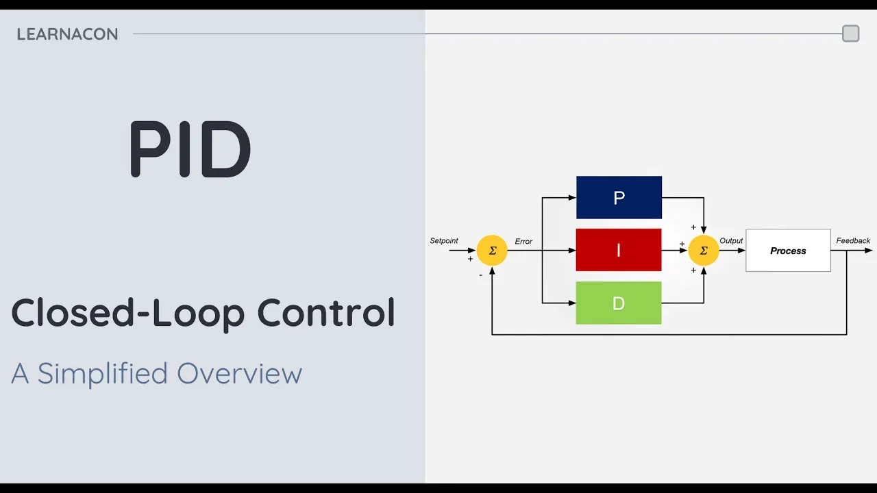
PID (Proportional-Integral-Derivative) closed-loop control is a fundamental feedback mechanism in industrial automation that automatically regulates systems by continuously comparing the desired set point with the actual process variable to calculate an error, then applying three correction strategies: Proportional (reacts instantly to current error), Integral (eliminates steady-state error by accumulating past errors), and Derivative (predicts future error trends to prevent overshoot); the effectiveness of PID control depends on proper tuning of these three components to achieve fast, accurate, and stable system response without oscillation or instability.

The closed loop transfer function is T(s) = G(s) / (1 + G(s)H(s)), where the denominator is the characteristic equation. Poles determine stability: left half-plane poles indicate stable systems. PID controllers (Proportional, Integral, Derivative) are widely used because they are simple, robust, and effective. The proportional term responds to error magnitude, the integral term eliminates steady state error, and the derivative term anticipates future errors.

Closed-loop control systems consist of setpoint, controller, process, and sensor. The output signal is the controlled variable (e.g., temperature), while the manipulated variable affects the process. PID control combines Proportional (responds to current error), Integral (eliminates steady-state error), and Derivative (predicts future error) actions. Continuous control includes P, I, D, PI, PD, and PID; discontinuous includes On-Off, Multi-position, and Discontinuous control.
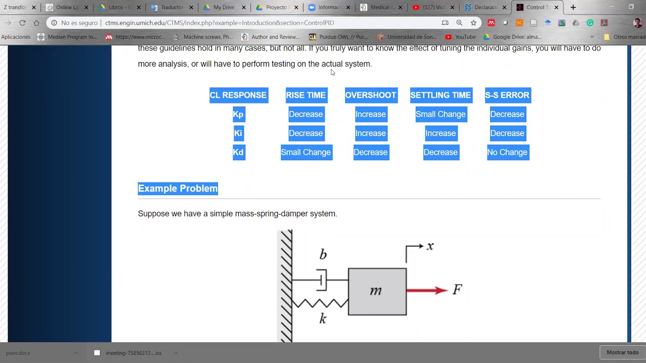
A simple closed-loop control system consists of a plant (such as an electric motor), a controller (which can be PID), and feedback. In the ideal case with a perfect sensor, the feedback is unitary, meaning the entire output signal is transferred without noise or disturbance to the input. The controller compares the desired reference with the actual output to generate an error signal, which is then processed to produce a control signal that drives the plant. The PID controller is mathematically represented as: u(t) = Kp*e(t) + Ki*∫e(t)dt + Kd*de(t)/dt. In the Laplace domain, this becomes: U(s) = Kp*E(s) + Ki*E(s)/s + Kd*s*E(s). The gains Kp, Ki, and Kd can be thought of as adjustable potentiometers that are tuned to achieve desired system performance.
Maze-Solving Algorithms: Implementing classical routing algorithms such as the Flood Fill, Bellman-Ford, or Depth-First Search (DFS) for rapid maze exploration and path optimization.

This segment introduces and compares five maze-solving algorithms. The Random Mouse algorithm randomly chooses directions at intersections but fails on large mazes. Wall Follower keeps one hand on the wall until reaching the exit, working well for solvable mazes. Dead End Filling fills dead ends until only the solution remains, visually impressive but computationally expensive. Dijkstra's algorithm finds shortest paths by selecting nodes with smallest cumulative distance. A* combines actual cost with estimated remaining distance to find optimal paths. Google Maps uses both Dijkstra's and A* for route finding.

Different search algorithms serve different purposes in maze solving depending on requirements. Depth-First Search (DFS) explores as far as possible along each branch before backtracking, which can find a solution quickly but may not find the shortest path. Left-Hand Rule follows a wall-following heuristic suitable for human-like navigation. Dijkstra's algorithm finds the shortest path in weighted graphs by always expanding the lowest-cost node first. A* combines heuristic estimates with actual costs for more efficient shortest-path finding in complex mazes.

Micromouse competitors use various algorithms to solve mazes. Wall-following works for simple mazes but fails with freestanding walls. Depth-first search runs as deep as possible before backtracking, eventually finding the goal but not necessarily the shortest path. Breadth-first search finds the shortest path by checking all options at each intersection but requires extensive backtracking. The floodfill algorithm, most popular today, makes optimistic journeys assuming no walls exist, then updates the map when hitting walls. It marks distances from every square to the goal, following decreasing numbers. While not guaranteed optimal on first pass, it efficiently finds the best path by treating return trips as new searches.

Early maze solvers used wall-following, which failed when goals moved away from walls. Depth-first search explores deeply before backtracking but may miss shortcuts. Breadth-first search guarantees shortest paths but wastes time rerunning paths. Flood-fill emerged as the dominant strategy, making optimistic journeys and updating paths when walls are encountered. The algorithm treats return trips as new journeys, efficiently discovering optimal paths while avoiding exhaustive exploration.

This comprehensive lecture covers the complete landscape of maze-solving algorithms for micromouse robots, progressing from basic to advanced techniques. Dead reckoning serves as the foundational approach where robots move forward until hitting walls, then turn—effective for collision avoidance but incapable of finding optimal paths. Wall following (left wall following) improves upon this by having robots consistently follow one wall, solving simple connected mazes 100% of the time but failing in complex configurations. Flood fill emerges as the sophisticated solution, finding the shortest path by continually updating distance values as robots learn about the maze. The algorithm uses Manhattan distance (horizontal and vertical moves only, like navigating city streets) rather than Euclidean distance, since diagonal movement through walls is impossible. The water flow analogy visualizes how distance values propagate through the maze, with water naturally spreading outward from the goal to fill cells in order of increasing distance. Technical implementation uses queue data structures operating on first-in-first-out principles, with systematic steps for processing cells and updating distances. Maze representation requires coordinate systems, 2D arrays for tracking horizontal and vertical walls, and 2D arrays for storing Manhattan distances. Debugging relies on print statements showing the robot's state and decision-making process. The robot knows it has reached the center when its coordinates match predefined goal coordinates.
Sensor Fusion and Wall Detection: Integrating infrared (IR) distance sensors or Time-of-Flight (ToF) sensors with the drivetrain to prevent wall collisions and correct odometry errors.

Combining a 2D LIDAR with ultrasonic sensors pointing in the driving direction creates a more robust obstacle avoidance system. Ultrasonic sensors have a wider opening angle (about 30 degrees) and can detect small obstacles on the ground that LIDAR misses. A system using at least five ultrasonic sensors would likely outperform a single LIDAR for comprehensive obstacle detection. However, even a combination of three sensors covering 90 degrees cannot solve the long wall detection problem, requiring full 180-degree coverage.

Sensors allow players to detect enemies through walls and obstacles. This provides tactical advantages by revealing enemy positions that would otherwise be hidden, enabling players to plan their movements and attacks accordingly.

Ultrasonic sensors measure the distance between the robot and walls by emitting sound waves and calculating the time for the echo to return. The robot uses three ultrasonic sensors (front, left, and right) to detect walls. When the nearest wall is on the left, the robot turns right, and vice versa. This allows the robot to navigate around walls effectively.
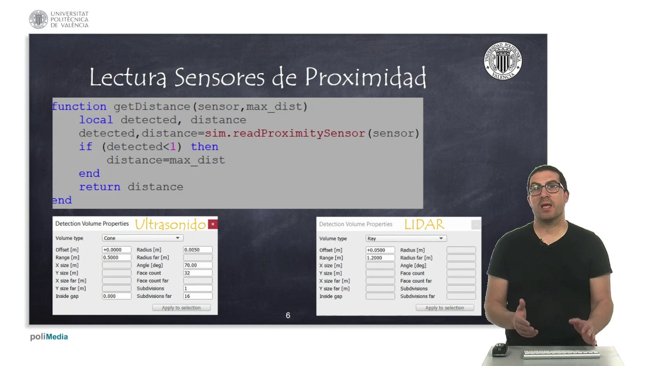
This section covers proximity sensor integration and wall detection logic. Proximity sensors (ultrasonic or LiDAR) provide distance readings through a sensor manager function, with 'max_dist' ensuring values between 0 and maximum range. Wall detection compares measured distances to expected values using tolerance thresholds to account for sensor inaccuracies. The 'walk' function returns true when the absolute difference between measured and expected distances falls below the tolerance. Robot construction parameters (wheel radius, sensor separation, wheel-to-center distance) are essential for accurate wall detection and maneuver calculations.

The movement sensor can detect players through walls and at any height, meaning it does not require a direct line of sight to function. The sensor activates when a player enters its detection radius and deactivates when a player leaves the radius. The sensor remains active throughout the entire round until it detects someone or the round ends. The sensor can be placed in various locations including corners, entry points, and elevated positions, and it will detect players regardless of their position relative to the sensor. The sensor works through any wall material and at any height, making it versatile for various tactical placements.
Advanced Embedded Firmware Design: Developing interrupt-driven software architectures to handle real-time encoder counts, sensor readings, and motor PWM updates concurrently.
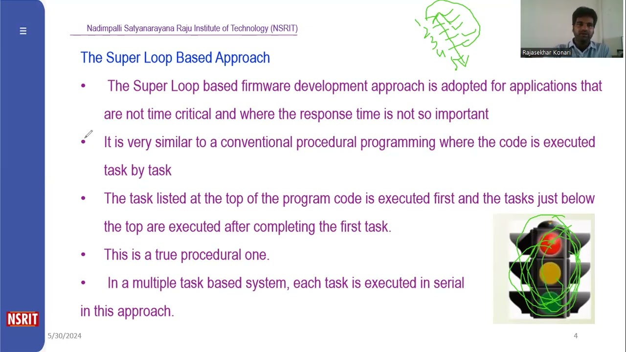
Embedded firmware design employs two primary approaches: the conventional super loop method, which sequentially executes tasks in a fixed order without an operating system and is suitable for low-cost, non-time-critical applications like electronic toys; and the embedded operating system based approach, which uses real-time operating systems (RTOS) such as VxWorks, ThreadX, or MicroC/OS-III to enable preemptive multitasking, flexible resource scheduling, and predictable event response for more complex embedded applications.

Embedded system design follows a systematic process: documenting characteristics and quality attributes, determining application/domain specificity, identifying hardware/software requirements, and developing program models using data flow graphs, state machines, or sequential models. Embedded firmware serves as the 'master brain' that controls hardware peripherals through code. Firmware imparts intelligence to embedded systems through a one-time process that can occur after fabrication or later. Successful firmware development requires understanding hardware components, memory maps, register configurations, and programming languages. The firmware enables products to function properly until hardware breakdown or firmware corruption occurs.

This extensive section covers advanced embedded system development methodologies. Hardware-software co-design requires integrated collaboration between engineers through model selection, architecture selection, language selection (VHDL/Verilog for hardware, C++/Java for software), and requirement partitioning. Computational models for representing processes include data flow graphs, control data flow graphs with conditions, state machine models with state transitions, sequential program models with timing logic, concurrent communication process models, and object-oriented models using inheritance. Firmware combines hardware and software characteristics, residing on microchips with binary-coded instructions. Design approaches include conventional procedure-based sequential execution and operating system-based designs (general-purpose for non-real-time applications, RTOS for real-time event processing). Programming languages range from assembly level (labels, op codes, operands) offering high performance but requiring expertise, to high-level languages (C, C++, Java) providing abstraction and portability. Embedded C differs from standard C in hardware dependence and compiler specificity. The compilation process involves assemblers, linkers, and locators converting source code to executable formats. Compilers target same-platform execution while cross-compilers support multi-platform development.
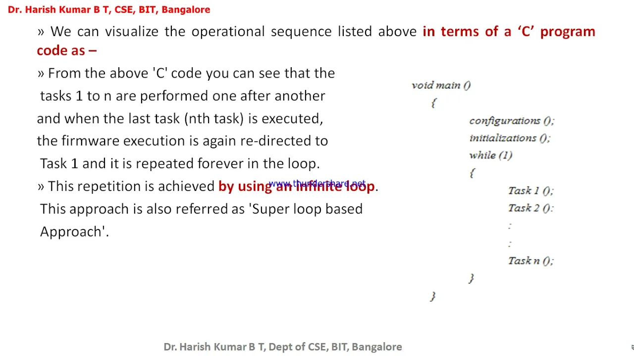
Embedded firmware is the controlling algorithm permanently stored in read-only memory (ROM) that manages hardware peripherals in embedded systems. Effective firmware development requires understanding hardware components, memory maps, register configurations, and interrupt architectures, along with proficiency in programming languages like assembly or C/C++. Two primary design approaches exist: the super loop (procedural/sequential) approach, which executes tasks one after another in a fixed sequence without an operating system and is suitable for non-time-critical low-cost applications; and the embedded operating system (RTOS) approach, which enables preemptive multitasking for real-time response requirements. Firmware development languages range from target-processor-specific assembly language to controller-independent high-level languages like C, C++, and Java, with hybrid approaches also being common.

Embedded firmware design employs two primary approaches: the super loop based approach, which uses an infinite loop to sequentially execute tasks in a fixed order without an operating system, suitable for non-time-critical applications but prone to system-wide crashes if any single task fails; and the embedded operating system based approach, which utilizes either general-purpose operating systems (like Windows/Linux) or real-time operating systems (RTOS) with pre-emptive scheduling to provide better reliability, real-time responsiveness, and task isolation for more demanding embedded applications.
PCB Assembly
0:00- 1
Soldered core components onto the board.
- 2
Combined SMD and through-hole soldering techniques.
- 3
Successfully powered and tested the microcontroller.
Algorithm-First Pedagogy: Simulation and Off-the-Shelf Hardware
While building a Micromouse from scratch—involving SMD soldering, custom drivetrains, and encoder integration—offers deep hardware insights, many robotics educators advocate for an "algorithm-first" approach. This perspective argues that the steep learning curve and high failure rate of custom hardware troubleshooting distract from the core computer science concepts of maze-solving, such as flood-fill algorithms, pathfinding, and decision-making. By utilizing high-fidelity simulators or pre-assembled modular robot kits, students can immediately engage with complex navigation and control theory. This minimizes the risk of hardware-induced errors (like cold solder joints or misaligned encoders) ruining the learning experience and democratizes access for students without specialized electronics labs.
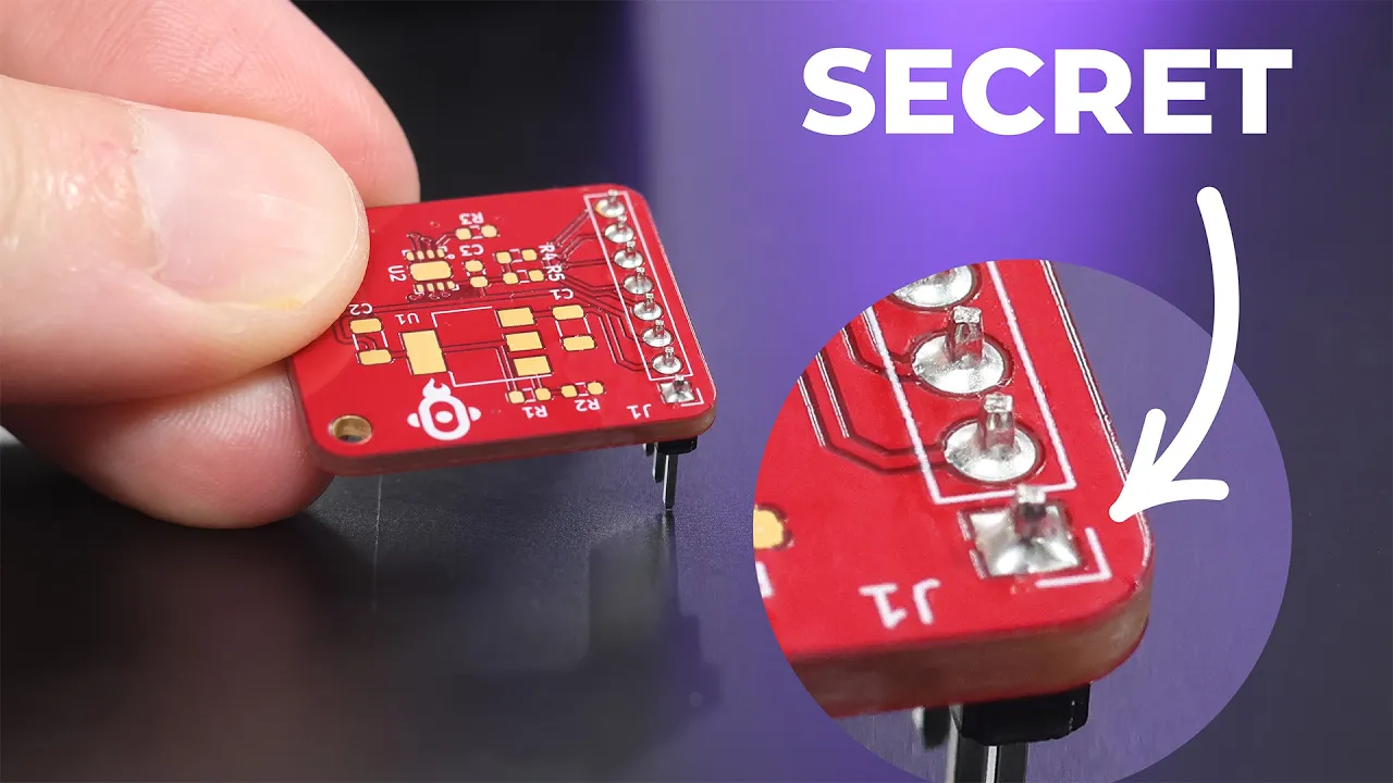
[Music] all right welcome back to part two out of three for the micro mouse series this time we're going to be focusing more on the build so last time was just an introduction to the different parts and a little bit about the micromass project this time we're going to be putting on the peripherals and then just testing each one of those out so we're gonna get a working micro mouse at the end of this and also we're gonna work through some of the bugs for that and my solutions around it so thank you guys for joining me on this process and i hope you guys enjoy it my dad got these like magnifying lenses that he uses for fly fishing i'm gonna give these a try because i have to like solder all these little components to the pcb yeah let's give these a try oh my god [Music] i first soldered on resistors and capacitors into the power input so that we can turn on the mcu and see if it works and i'll show you guys this a little bit later in the video so here's a nice little close-up of the board you can see that for the smaller components i'm using smd soldering so surface mount device soldering and then for the larger devices like this button i'm using through-hole soldering so the pins go through the board and i solder them on the other side [Music] finally here's me testing out the board and you can see that it works nice now we can go on to the next step the drivetrain [Music] [Applause] i 3d printed a motor stand so the motors can sit a little bit higher and give some room for the encoders and the wheel the motor mount the motors and the encoders will stand in this middle section of the mouse right here [Music] all right so i've programmed it and now we're just gonna test it out on this table here whoa okay all right nice um up next we're going to be putting these encoder boards so that we understand how far and how fast they're moving so yeah that'd be cool all right let's keep it up [Music] [Music] sometimes all i think about is [Music] all right guys thank you so much for watching part two of the micromast series the build in part three we'll be testing it out and making sure it can actually solve the maze so thank you guys so much for tuning in and we'll see you on the next one never peace
Up Next

Uncovering a Lost Tom Roberts Masterpiece: Art Authentication
@PerspectiveArts
323.4K views•2023-02-11

Triumph of Orthodoxy Icon: Byzantine Art & History Explained
@BenCallan
2.1K views•2024-08-06

FastAPI vs Flask vs Django: Choosing the Right Python Web Framework
@TechWithTim
302.5K views•2024-05-26

Game of Thrones Opening Credits: A Cinematic Analysis
@gameofthrones
46.3M views•2011-04-18
Related Study Plans & Knowledge Roadmaps
Structured learning paths in General & Interdisciplinary Studies