








![[KAU 동역학] 개요(Overview)](https://i.ytimg.com/vi/hGMnxytDtYk/maxresdefault.jpg)












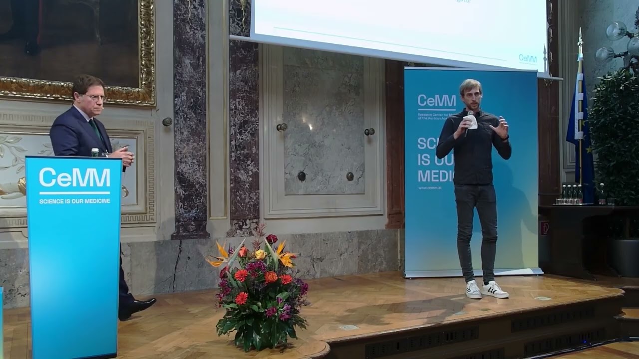
In avian gastrulation, the embryo transforms from a circular disc into a pear-shaped structure through two independent kinematic modules: Repeller 1 controls embryo size through a tug-of-war between extraembryonic epiboly and epical constriction, while Repeller 2 controls embryo shape through mesendodermal active intercalation; these modules can be independently modulated experimentally, demonstrating that complex morphogenetic processes can be decomposed into mechanically distinct, controllable units.
Tissue Flow Modularity in Avian Gastrulation | Serra Lab Talk
Added:Fundamentals of avian embryonic development, particularly the stages of gastrulation, primitive streak formation, and germ layer specification.
Basic concepts in tissue mechanics and biophysics, such as how collective cell sheets exhibit fluid-like, viscoelastic properties during morphogenesis.
The principles of collective cell migration, specifically how individual cell behaviors coordinate to drive large-scale tissue deformation.
An understanding of kinematics (the mathematical description of motion) versus dynamics (the forces that cause motion) in physical systems.
Advanced theories of active matter physics, analyzing biological tissues as self-propelled, non-equilibrium thermodynamic systems.
Mathematical and computational modeling techniques, such as continuum mechanics and vertex models, used to simulate embryonic tissue flow.
Evolutionary developmental biology (Evo-Devo) investigations into how variations in these kinematic units drive morphological diversity across different amniote species.
Applications in bioengineering and regenerative medicine, specifically using tissue flow modularity principles to guide the self-organization of synthetic organoids.
267 views0likes26:01Original Release: 2024-09-16
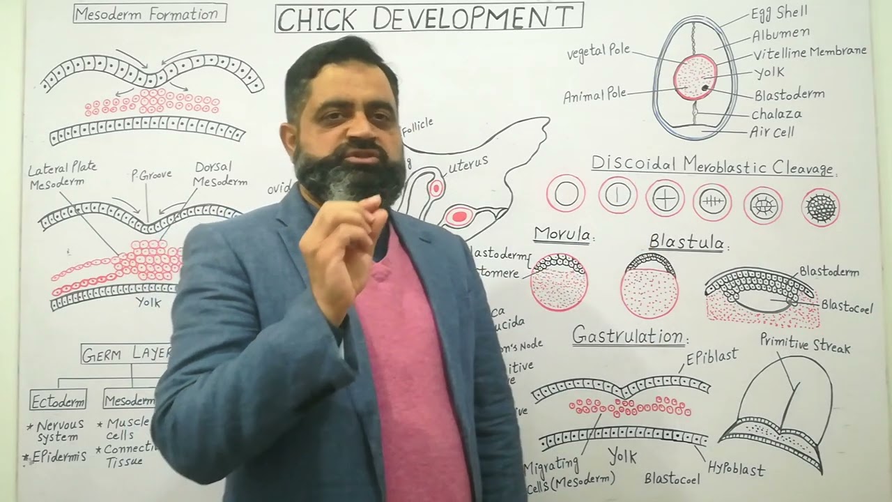
yes thank you so hi everyone and um I'd like to thank the organizers for this uh wonderful series and for giving me the opportunity to speak um today I will be talking about control of uh tissue flows and actually uncovering also modularities of tissue flows in aan gastation this work was led by Alex Plum is's a PhD student in my group a guo posto Serano postto in the steventon lab at Cambridge and ke be group at University of dandi um so it's very well known sorry if some videos will not play the my PowerPoint just updated now five minutes ago as an unpleasant surprise but it's very clear and well known that in early development cells will undergo large scale motion at actually the embryo scale and uh across model systems and today we'll be focusing on the chick or avian gastrulation which is the example on the right and uh in the chick gastr at very early stage of development the embryo is just a thin disc is 3 mm wide there are about 50,000 cells and this disc sits on top of the yolk that you can actually visually see cracking an egg and in the first 15 hours of development the embryo transforms from a circle into a peir shaped structure and if you image this uh disc of 50,000 cells you can see a very um vigorous multicellular flows and today I want to sort of touch based on two concepts the first one is trying to understand how the embryo controls its geometry how does it transform from a circle into a pair shaped structure in this first 15 hours of development and the second question I want to try to address is whether these spot temporal complex flows which are typical of basically any morphogenetic process not to the specific to the cheek embryo can we actually decompose them in kinematic units that perhaps have different developmental biology functionality uh they can they have different origin or mechanistic origin and perhaps can be controlled uh independently just to give you uh a perspective of Avan morphogenesis will'll be looking only at the first 15 hours of development while the full evolution of uh this developmental process takes about 20 days so when you put this embryo under a confocal microscope you can basically CDC uh or extract velocity Fields using pav um and uh to study this multicellular flows you can either use aian approaches which is for instance looking at velocities at fixed aian coordinates and then you get something like this so which has basically streamlines or you know velocity snapshots at different times uh however thisan approaches some bottlenecks that are or problems that have been recognized for instance in Contin mechanics and the F most important one is being uh frame dependent that means for instance that if I now change the coordinate system I want to use to describe it this motion the motion of cell and the origin of this coordinate system is pretty arbitrary or for instance if you have an embryo that slightly drifts under your microscope the structures of these velocities will completely change okay so in alternative to thisan approach is instead looking at lran approaches which is instead of looking at the embryo from a six grade you instead look at the motion and the formation of the embryo so basically you look at cell trucks or tracks or trajectories of patches of tissue so you start at the particular initial condition X zero You observe the system for a certain time interval depending on your experiment this blob has been now moved to a different position and on top of trajectories you can also compute the deformation gradient which is just the Jacobian of this flow map or trajectory map if you will and that basically is going to tell you for instance in initial disc of Cs we transform into an ellipsoid and it's going to tell you what's what are the directions maximum stretching Etc and uh this if you want to visualize it very also very simple you can just overlay a lran grid that deforms with uh your um your embryo and that gives you a view of how the tissue deforms as uh it um evolves over time now the deformation gradient is a tensor which means that for any initial condition of of your embryo domain and for any time interval you're exploring this is going to be a matrix so it's very hard to visualize a very relevant information that you can extract from this tensor is its largest singular value so you have a tensor for any point of your domain and any time interval you extract the scalar field which is the largest singular value and that tells you the following information assume for instance you are here this is your initial or initial embryo location that you want to probe this largest singular value will tell you how much initially near by will maximally separate so you are initially closed at different sides of this basically line which is an I value of this largest singular value and basically tells you that if you have a lot if you have a very large largest singular value in this spatial domain that means that cells that will eventually start close at the opposite side of these lines will separate maximally so you can imagine that regions where this Lambda 2 is very high will demarcate repellers in the embryo those are regions where cells start initially close at the opposite sides of this region and then will maximally separate over time so now you can uh calculate this um quantity in the data that I just showed you can basically iterate over increasing time interval to see how these structures evolved dynamically and the CH estation data will um basically be composed of two repellers there is going to be a repeller number one and a repeller number two over this 15 hours of development and I'm going to explain the meaning of these two repellers in a second so the second thing you can do similarly instead of looking at repulsion you can also look at convergence which is looking at another singular value of this deformation gradient you can say what are the regions that will most strongly attract cells that will initially start far away from each other and that's basically going to be another structure another regions where a scalar field will be high which is this this structure here so this is going to be an attractor which in this Chi gast case corresponds to basically the Primitive streak this is a region where cell will converge in this dis and then it will eventually Ingress into the third dimension to start the formation of the other germ layers so basically what we did we transformed a set of spal temporal velocities that are frame dependent into three structures one repeller repeller number one that basically splits all the extra embrionic cells from the embryonic cells whatever is within the repeller number one or inside repeller number one is what going to form the embryo the rest are sort of auxiliary cells that are made of extra embrionic cells then you have a one attractor which is basically the prim streck this is where cell will converge and then Ingress leaving this epithelium and then there is repeller number two that basically splits the anterior part from the posterior part of the primi streak or the attractor so basically what we did we compressed this special temporal velocities in three kinematic units two repellers and one attractor and what we did conceptually we got rid of all the frame dependent information and we retain also the objective deformation if you think of deformation you can also think of the rate of strain tensor which is accounting for instantaneous deformation or deformation rates if you will however when you have a morphogenetic process you want to understand how the tissue deforms cumulatively as it moves okay that's basically lran that's the difference between the rate of strain and this dyamic morphos skeleton and then as we said before the deformation gradient has a lot of information because it has a tensor for any point in your domain so what we did we just extract the highest deformation in terms of contraction and Com or or repulsion that's basically what we did so we transform this speci temper fro in these three kinematic units Beyond describing gastrulation we apply this technique now to several model system from drosophila to zebrafish and recently we found also that later stages in chick development and also in rosopa we found that the emergence of repellers may be important or may be implicated in early Sate bifurcation just as a flashing this information but what I want to talk about today is instead trying to address a few new questions with this technique so as I said CH gastrulation can be compressed into two repellers and one attractor and what we want to understand now is what are the mechanistic origins of uh these repellers that we we found uh can we modulate independently this depend are they modular are they independent how does actually the embryo changes shape from its circular initial geometry to a pair shaped geometry at later stages and can we control these repellers independently to do that we need to understand a little bit of the cell behaviors and then the mechanistic origins of the cell behaviors or the drivers of the cell behaviors and uh as we seen in the earlier slides we know that at the beginning of the development the embryo is a dis there's going to be three regions in this embryo the extra embrionic territory then there is going to be the embryo proper which is what's going to be inside the embryo and we know that there is going to be a repeller that splits these two and then within the embryo proper there are different cell types in the posterior which are called mism now if you look at this 15 hours later this embryo has expanded because the edge cells are basically pulling the extra embrionic tissue and also all the embryo then the embryo proper is transform into first shape and the mism has now converged to the midline which is the prim District the attractor and then is going to be ingressing the third dimension and if you want to look this in a microscope you can see that this motion is driven by active intercalation in the mesoderm you can have appical constriction throughout the embryo proper and active celling ression in the streak so in the streak there's going to be cells that convert to the strict vactive intercalation then they undergo EMT and they will basically pull the nearby tissue so they will apply a very strong active force in this developmental process and the last term is or the last process sorry is about epibole so these Edge cells uh they basically um with myosin will basically adhere to the Ving membrane they will exert traction forces and will basically pull all this uh extra embrionic territory which is attached also to the embryonic territory so those are basically the cell behaviors and all these process are B driven by myosin motor and this is an experimental image in which you can see in red actin and in cyan phosphorated myosin 2 uh I I I guess and you can see that the embryo has different regions some are actives and some are passive for instance if you look at EDG cells you see that edge cells are very enriched of myosin because they Den myosin to undergo EPO there is instead the extra embrionic region that has very little myosin is basically devoided of myosin so so is more more of a passive uh tissue in this uh epithelium uh there is then the embryo proper that has myosin but not as much as the primi streak or the mism regions where there is even more myosin and on top of myosin intensity you can also quantify basically myosin an isotropy or if you will actomyosin cables so you can basically do fast transform on these images and you can IM you can basically measure if you have atomizing cables that are oriented so there's going to be an orientation in this segment here and there's going to be also a length of the segments that tells you how much nearby cells have the same orientation in the aomine cables so those are basically what people call multicellular uh cables okay so basically with this ingredients with this quantification we have everything we we need to quantify or model the active stresses specifically we have the myin activity a scater field then we have a nematic tensor that accounts for the presence of cables so as is going to be the cable alignment or the nematic order parameter if you don't have cable s is equal to zero if you have very aligned cable s is close to one uh and the f is just the cable orientation so with this uh informations you can now build an active stress so there's going to be M that tells you the amount of active stress uh I mean the amount of active myosin and then Alpha just converts Myas into stress and then you have an is an identity tensor that accounts for the isotropic active stress that is reflecting basically AAL constriction and active ingression and instead Q the nomatic tensor accounts for the active intercalation Okay so this is just the active stress and uh this system is extremely viscous is sp like a long time scales because you have basically motion that are uh very large scale and there's a lot of you know neighbor exchange therefore we can sort of say that simply that the Divergence of the active stress plus the Divergence of the passive stress or the viscous stress is equal to zero that's basically the force balance and the viscous stress they have basically the sheer force but also a force due to compressibility because this tissue is compressible it expands in area but also has to accommodate in ression so from this first equation very simply you can read that if you know the distribution of M and Q you can identify immediately the velocity of the tissue at any time instance so to close the system then you need an equation for M and an equation for Q so the equation for m is about the myosin Dynamic is also um simple so if you have a cell with a lot of phosphorated myosin and you move you're going to carry the myosin with you that's the advection myosin or activated myosin can be activated by from an available pool of myosin that's basically the activation term and myosin can also or the activated myosin can also detach from acting in a tension dependent manner this is the Detachment contribution is me sense itive the details of this are basically well explained in in the reference and then the last term is about myosin induction Thea tension propagation which basically reflects the expectation that if I a myosin Cable anding cable and I pull I will put my nearby Junction under tension and if I put them under tensions due to mechanos sensitivity they will recruit more myosin and that's basically what you get uh what what basically is been described by this directed lapasan and the derivation of this expression is again detailed in the in the paper so very interesting property of this equation is about the fact that this mining equation as as um instabilities this is what we found in an earlier work and we also validated experimentally and specifically this PD has a stable fixed point of IM myosin which is basically what likely happens in the embryo proper or in the pr streak where we have a lot of where you have a lot of minine there is also another fixed point in um in the lower of myosin so basically very little myosin which is likely what happen in the extra embrionic region when there is no myosin um and both these two are stable while there is an intermediate fix point which is unstable which is what we believe is where actually the embryo is operating throughout gastrulation because experiments show that actually there is a strong increase is in myosin from hh1 to hh3 okay so the last ingredient that we need is the evolution equation for Q this is very similar to the active met equation so you have the advection term because if you have cable and Order you're going to transport them with advection uh you're going to have that cables are rotated by vorticity so that's basically encoded in the spin tensor Omega here uh but there is also a sheer contribution because you know Shear rates or Shear rotation can either construct or destroy order this is also something known in in active matter that's this term here however if you just use these three terms this this this these equations are not is not sufficient to recapitulate Observation because convergent extension and specifically the sheer contribution self destroys order and therefore you need a mechanism to sustain order to sustain basically convergent extension and that's what is uh um described in this term which is the active alignment this active alignment basically reflects this expectation that if you have a little bit of nematic order so s is greater than zero naming I have cable and you have Milos in that regions these cables will contract right so this cable will contract and therefore will create long range order so will increase basically the S at that particular location that's basically what we call Active alignment and this was also found recently in from the shiman group in vertex model so they basically found that to have sustained convergent extension you need a mechanism to basically generate order which otherwise would be destroyed by for instance um uh sheer um destruction of Bas alignment and the last term is something which is basically happening everywhere in the epithelium because there are a lot of random intercalation and ingression these processes they will all in general destroy order so that's basically the passive uh um relaxation term okay so now we have this set of equations uh what do we need to solve the problem we need basically boundary conditions so boundary condition for the force balance is very simple you just need EPO velocity uh on the due to Theo velocity is just a der boundary condition normal velocity at the boundary of our domain we can get these numbers from experiments because we can measure the P velocity and then we use no flux for M and Q and the last ingredient we need are the initial condition for M and Q and we know basically two important ingredients the first one also as we've seen before that is that the embryo has more myosin than the extra embrionic region so in the embryo there is more myosin we've seen also in the actin and myosin two plots before and the second thing is that the cables are actually at the onset of gastr relations are more concentrated in the posterior where the mism is in this basically posterior region of the embryo and in this posterior region at the beginning because these cells are mism they also have more myosin so basically the boundary condition the initial condition for the for the flow is the following for the model is the following so we have low myosin in the extra embrionic region higher myosin in the embryo proper and a little higher myosin in the posterior and then you have more cable aligned in the posterior this is basically what we can get from experiments and the rest is just boundary condition from epipole and I want to basically emphasize something very important which is that the boundary the initial boundary between embryonic and extra embrionic region is just a circle at the beginning and now what we're going to do we're going to evolve this PD with this initial condition and Boundary condition and we will see how this B boundary will sort of self organize and evolve but I want to make sure that we understand that we are not imposing anything on this boundary the boundary of the PD is just here so we the way this white curve which is the embryonic boundary will evolve is just a result of self-organized result of the model we're not imposing anything on its Evolution so the question now is I have the model we have the the initial condition conditions can the model reproduce What happens in the next 15 hours of development you have about five minutes just to let you know oh okay okay um okay so basically that's that's basically the model uh you can um evolve this basically U model you can see the velocity field the Divergence the evolution of the boundary of the embryo that is basically changing from a circle to a pair shape this matches experiments in terms of distribution of velocity and diers you can also measure the uh or describe the evolution of active isotropic stress so this shows basically that the myosin increases in the embryonic region increases even more in the um in the mism and if you basically match it with experimental observation it's pretty much um similar uh Evolution you can also um show the distribution of the vactive an isotropic stress this is basically M * Q which is the nematic order parameters times the orientation and this also matches observation which is basically having eventually cables that are perpendicular to the strak where there is a lot of order perpendicular to the strak and this is basically what you can get if you have the same quantification in experiments what I want to do now I want to go through the um Dynamic morphos sceleton and have a lran assessment of these results which is I can the lran grid with the model velocity this is what you get in terms of uh a deform lran grid you can do the same using a velocity from exper ments you get basically that the embryo transforms from a circle into a pair shape and you can also recapitulate the repellers so you're going to have repeller number one that splits embryonic and exter embrionic and repeller number two that splits the anterior part and the posterior part and similarly you can get the same using the experimental velocity what we want to do now we want to understand if these repellers have different mechanistic Origins so what we want to we want to try to knock them out separately in model and experiments so the first one is eliminating repeller number two we we hypothesize that repeller number two arises from the mism the active intercalation from the mism so in the model we just remove the bump of myosin in the posterior and we left we let the model evolve with exactly the same initial in boundary condition and this model predicts that the embryo doesn't change shape if you remove mism you eliminate repeller two but retain repeller one and if you do now the same uh knockout experimentally any beating mesoderm induction you get exactly the same result which is basically the embryo does not change shape remains circular retains repeller number one but eliminates repeller number two okay so then the second thing we wanted to eliminate repairer number one and to do that we hypothesize that repairer number one arises from a tag of war between extra embrionic EPO and epical constriction so we said let's block EPO which in the model means uh setting the velocity the boundary velocity equal to zero you solve the model basically leaving everything else unaltered you see that the embryo still changes shape you retain repeller number two but um um eliminate completely repeller number one so now guo what he did he basically to implement this he basically burned the vitalin membrane so he cized the vialing membrane the cells cannot really exert any more traction because there is no Ving membrane and therefore you can block EPO compared to the the white Ty so when you do that that experimentally you still see indeed as in the model that the the the embryo still changes shape you retain the repeller number two but eliminate completely repeller number one basically in Vivo and of course you can now do the combined perturbation blocking both epiboly and mism and you see basically that you can block and eliminate leair number two and reper number one together in the model and in the experiments so basically what we learned is that repair number one arises as a tag of war between extra embrionic EPO and epical constriction while repair number two arises from the active intercalation of the uh of the mism and what was interesting to understand and to see is that you can actually modulate and control these two kinematic modules independently in Vivo consistent with the with experiment so basically in summary in this uh short talk we talked about the control and modulation of repellers in previous works we were also able to modulate the geometry of the attractor which is the Primitive streak we transformed it from a from a line to a circle to a point and to a thicker line mimicking or recapitulating um gastrulation modalities that are typical of other vertebrates in the cheek so in terms of mini summary of of this story is that we started with experiments with special temporal velocity we compressed those into their kinematic units the dynamic morphos skeleton uh and then we were able to build a minimal model minimal active met model can that can reproduce these kinematic units and then using these models and this compression we able to devise uh model inspired perturbation that were able to knock out this kinematic units independently so that's basically my summary slide and perhaps the interesting part that I didn't say so far is that basically repairer Number One controls the embryo size and are ostasis via the St of war between extraembryonic capo and igal constriction while repeller number two controls the embryo shape because we've seen that El ating re number two the um cheek ambo remains Circle and doesn't basically change shape and perhaps a speculation could be that because these are due to different mechanistic Origins that can actually be controlled and modulated in Vivo uh uh distinctly maybe this modularity could be helpful for evolvability of different aspects of chi gation thank you very much and perhaps advertise postto and and and and PhD student positions that we have in the group
Up Next
5:17
Mammalian Embryo Axis Specification | A-P & L-R Patterning
@amysaldana3109
6.6K views•2020-11-02

50:12
Bacterial Communication: Quorum Sensing and Biofilm Formation Explained
@JHUAAP
12.6K views•2011-06-28

5:35
Enteric Nervous System Explained: The Gut's Brain | Neurobiology Lecture
@alumniu6029
438 views•2018-09-12

7:08
Bacteriophages: Earth's Deadliest Killers and Future Antibiotics
@kurzgesagt
34.6M views•2018-05-13
Related Study Plans & Knowledge Roadmaps
Structured learning paths in Biology
biology
RNAi: Biogenesis, RISC & Gene Silencing
01Molecular Biology Foundations: DNA to Protein
02Introduction to RNA Interference (RNAi)
03Molecular Biogenesis of miRNA and siRNA
+ 2 more learning modules
10h5 modules
Explore Roadmap
biology
Mycorrhizae: Signaling, Biophysics & Ecology
01Foundations of Mycorrhizal Symbiosis
02Molecular Signaling and Root Colonization
03Biophysics and Bioenergetics of Nutrient Exchange
+ 1 more learning modules
11h4 modules
Explore Roadmap
biology
Circadian Clocks: TTFL, SCN & Periphery
01Foundations of Molecular Biology & Gene Expression
02Introduction to Chronobiology and Actograms
03The Core TTFL: Molecular Architecture of the Clock
+ 3 more learning modules
14h6 modules
Explore Roadmap
biology
Population Genetics: Math, Drift & Selection
01Genetic & Probability Foundations
02The Hardy-Weinberg Principle and Baseline Models
03Mathematical Modeling of Natural Selection
+ 3 more learning modules
18h6 modules
Explore Roadmap