










![dr. V. Petrík: Robotika (B3B33ROB1) – 06 [30. 10. 2023, ZS 23/24]](https://i.ytimg.com/vi/nv-07JsesXQ/maxresdefault.jpg)



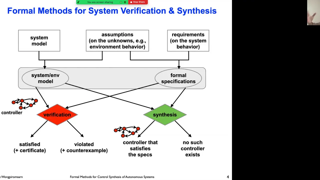
![Serwonapędy w przemyśle [Webinar] | Schneider Electric](https://i.ytimg.com/vi/Hle1-_TZi_A/sddefault.jpg)




![Multibody Dynamics [MAE 223] Fall 2017 Lecture 20](https://i.ytimg.com/vi/Oou3ZItxtjM/sddefault.jpg)






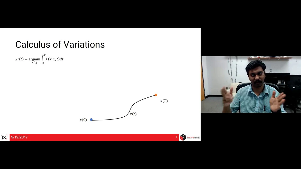
Trajectory generation determines how joint variables change as a function of time between waypoints, unlike path planning which only specifies endpoints; common methods include cubic polynomials (satisfying initial/final positions and velocities), quintic polynomials (adding initial/final accelerations), trapezoidal velocity profiles (linear segments with parabolic blends), and s-curve profiles (seven-segment profiles with constant jerk) which provide smooth motion by eliminating abrupt acceleration changes that cause mechanical stress and jerky behavior.
Trajectory Generation Methods for Robot Path Planning
Added:Fundamentals of kinematics, including the mathematical relationships between position, velocity, acceleration, and jerk.
Basic differential and integral calculus, essential for understanding rate of change and integration over time.
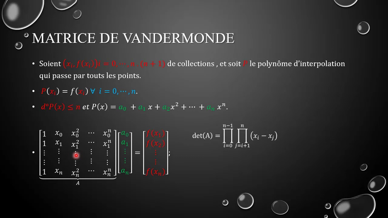
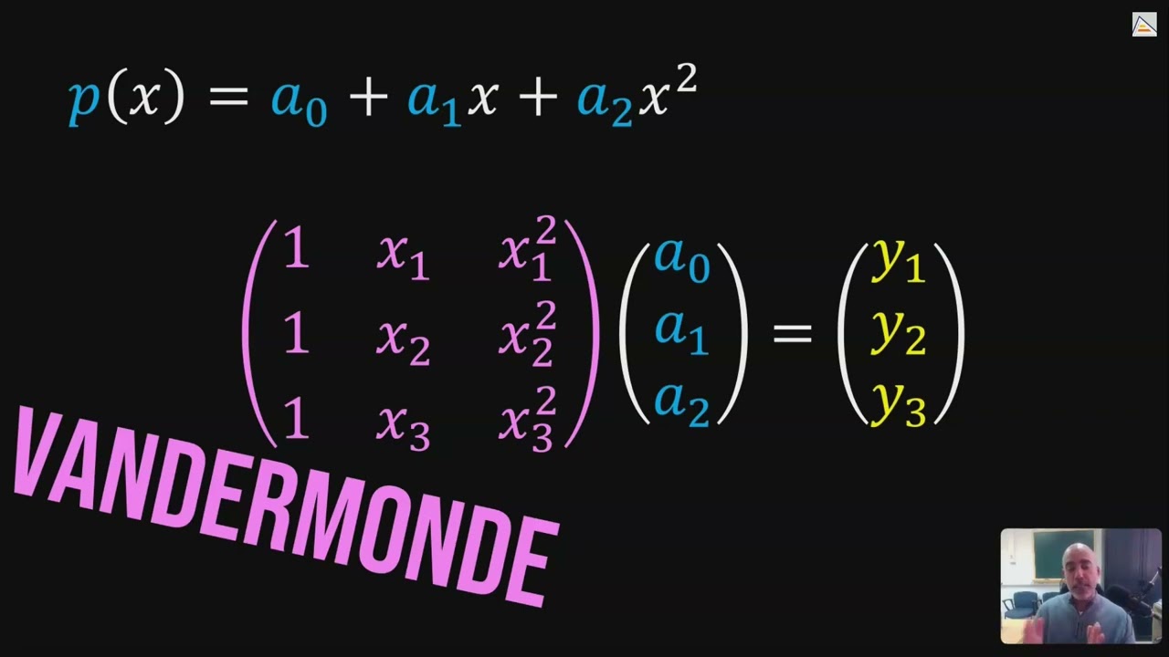
Polynomial interpolation and methods for solving systems of linear equations to determine curve coefficients.
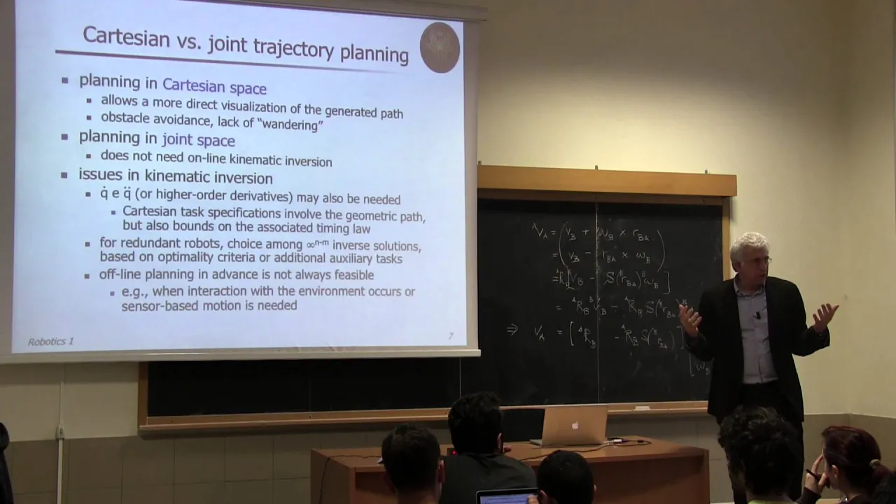
The conceptual distinction between geometric path planning (spatial coordinates) and trajectory generation (time-parameterized profiles).
Multi-axis trajectory synchronization to coordinate simultaneous movement across multiple robotic joints.
Advanced curve parameterization techniques, such as Bézier curves, B-splines, and NURBS, for complex path design.
Trajectory optimization methods aimed at minimizing energy consumption, execution time, or actuator wear.
Implementation of feedback control systems (e.g., PID or computed torque control) to accurately track generated trajectories.
Dynamic obstacle avoidance and real-time trajectory replanning in unstructured environments.
23.1K views473likes1:20:01Original Release: 2021-07-24
hello everyone as you know the path planning was really a non-parametric identification of the path right basically what you did you determined a bunch of waypoints and you tried to go from one way point to another and avoid collision but you never specified in path planning that when you have q values correct for each one of the waypoints you have not specified how the q and the joint variables would change as a function of time from one waypoint to another right so all you have was the end points just the end point q q1 and q2 or q0 and q final that's all you had how q changes versus time that was not discussed in path planning and that is the topic of trajectory generation so in trajectory generation i want to find q as a function of time what kind of time function i should choose for q if i only know the end points and you might say why is that any important because if i i'm sure that there is no collision happening what's the importance of q well you know if for example q corresponds to the angle of a joint right let's say it's a rotary joint then the time derivative of this q is what q dot which is the angular velocity omega and then what the time derivative of that is q double dot which is the angular acceleration or alpha correct and this angular acceleration does depend on what on the torque correct for example you know if it's theta double dot theta double dot or alpha is equal to what the torque divided by the mass moment of inertia i right or if it's like the um it's a prismatic joint then d double dot is equal to the force applied to the joint divided by the mass correct and you know you have physical limitations on the amount of the torque that a motor can generate or the force that a linear actuator can generate right they have limitations and so when you divide them by these numbers i or m your d or your theta double dots they have some max values correct right so if i wanna write it like this you have some maximum this is like a correct this is like a and this is like alpha there is some maximum acceleration and maximum what linear or angular acceleration you can have and also when you integrate those this guy can be either linear velocity or what angular velocity this guy will only also have some maximum correct you cannot expect from a motor to give you any rpm that you want and any torque that you want and you also know that the omega and torque for example for a motor they do depend on each other right as the rpm goes up the torque drops and vice versa so you have limitations physical limitations on the driving force or the driving torque behind your joint and that's why this function of q does matter because if you choose this q of t such that your angular acceleration or linear acceleration exceeds what the motor can give you then your robot cannot achieve the task right the way that you want for example let's say i want to go from my initial q value and let's say t naught is 0 or whatever and t f is 2 seconds and i want to go from initial q of 0 radians to final q of let's say 400 radians and the timing i have is from 0 to 2 seconds so in 2 seconds your joint has to rotate 400 radians which is on average 200 radians per second and if you multiply that by 60 over 2 pi correct you can convert it into rpm 60 over 2 pi is roughly 10 so 200 rpm means what means 2 200 radians per second means 2 000 rpm now can your motor give you such rpm maybe maybe not and also when you calculate your acceleration i'll show you angular acceleration maybe it shows that your maximum angular acceleration based on the uh inertia of the motor is going to be and the load of course right this is the inertia equivalent this torque is going to be let's say a hundred newton meters does your motor have that torque maybe maybe not so you have to know how these joint variables are changing versus time good so now that we know the importance of it how do we determine that so there are different ways depending on what is it that you want to control and what is it that you have what pieces of information you have then there are different methods what are the limitations and so on there are different methods for generating trajectories uh here we discuss two of them that are polynomial cubic and quintic and then there is one that is very common in a robotics application trapezoidal motion profile or you might also call it linear segment with parabolic blend okay so in terms of joint angle it's parabola line parabola in terms of velocity it's a trapezoidal okay and then finally we look at the s-curve which is a trapezoidal but it is smooth so here we need to look at a bunch of things the last thing i want to talk about before we start is the notion of jerk okay this jerk is a physical quantity and it is defined as time derivative of the acceleration okay so for example if it's theta double dot jerk is like the time derivative of theta double dot if it's a is like the derivative of a so the rate of change of acceleration the rate of change of acceleration whether it's linear or angular doesn't matter the rate of change of that we call it jerk and what does this one show really physically as the name says it's the uh jerk in the motion so if you ride for example in a taxi and the taxi what does have sudden stops slams on the brake and then when he starts moving he slams on the accelerator right so if you look at the acceleration plot versus time right let's say first the taxi is cruising so acceleration is zero then he boom slams on the brake and in a very short time he goes to a very big negative acceleration right and then what he um goes to zero speed and then um stays there stationary for some time then when he wants to start moving again boom slams on the accelerator and goes to a huge acceleration again right so if you look at this type of motion when you are sitting in the car you feel all of these changes in acceleration which is basically the changes in the forces applied to your body and if the forces that are applied to your body from the seats of the uh taxi you're not gonna feel any comfortable right you see one time the sit is pushing you the other time you are going to the windshield and so on and so forth right so that's what you felt or like when you go to this different rides in a theme park you see when the merry-go-round or anything like that is rotating this way and all of a sudden they what they stop and they switch the direction of rotation or it goes right you some of these rides if you have seen they go when they are also rotating they also go watts up and down and those changes in acceleration or the changes in the force will cause the jerk and the motion okay so this idea of jerk just wanted you to know about it because that is important to us so now let's talk about the polynomial uh functions for the trajectory right cubic and quintic so when is it that cubic polynomial is a good function to choose when you only have four values that you necessarily want to achieve what are they it's the joint variable at the beginning time it's the joint variable at the final time and then the joint velocity at the beginning and the final time right so all you know are the joint values at the beginning at the end and the joint velocities at the beginning and at the end and here we are just focusing on one variable so here q is not a vector it's just one variable but you can do this operation you can do this uh basically curve fitting right to each and every one of the joint variables right so if you have four joints and you call them q one q two three and four for each one of those cues you can apply a cubic polynomial like this so i say now this specific q is going to be a cubic polynomial so it has four coefficients unknown a naught a one a two and a three and this guy is gonna satisfy these four conditions for me why because it has four unknowns correct so we set it equal to this and then we apply this condition so we for t we apply t naught and set it equal to q at t naught then we for t again we apply t f and it is going to be q at t f then we take a time derivative from this and in that time derivative q dot which is what clearly you know q dot is going to be a one plus two a two t plus three a three t squared in that one again you plug in t naught and t final and the values for them you call them q naught q dot at t naught and q dot at t f and you will get four equations here are these four equations arranged in a matrix format where here this matrix on the left hand side this a matrix is a matrix with known values everything depends on time this is your unknown vector x which are the unknown coefficients and the right hand side is also a known vector based on the four given values so clearly from here your unknown vector x is gonna be what a inverse times b and once you have that you plug them back here you have now your q as a function of time so you made your q values parametric what is the parameter it is time okay and if you look at the way that the function is so at time tune t naught it is q naught q naught is this guy this is called q naught and t final it is q final and also the slopes at the beginning this initial slope here this initial slope if you call this angle for example alpha let's see if again [Music] so here that's the initial slope and this angle is alpha clearly alpha is tangent inverse of q dot at t naught and then you also have some final slope like this and again the angle of that with respect to the positive horizontal axis beta this is equal to tangent inverse of q dot at t final okay so you have the initial and final slope and initial and final value and it passes a cubic polynomial this is what you see and then as i said you can plot your q dot which is like this with the coefficients that you determine and you can also determine your what q double dots the acceleration terms which is going to be 2 a 2 plus six a three times t okay and so here i'm going to show you that in a matlab demo so these values i chosen is my initial time i chose it to be 0.5 final time 4.5 i go from pi over 6 to 4 pi over 6 so all i'm rotating is about 180 degrees i'm rotating 180 degrees in four seconds it's not such a big deal and my initial and final slopes are given as 0.5 and 0.2 i calculate my a and right hand side here is the same as b matrix get my coefficients get my q q dot q double dot and all i'm doing is plotting it right so here we go you can see q q dot and q double dot all of them as a function of time clearly you see your q starts at [Music] pi over 6 right at 30 degrees and goes to 7 pi over 6 right which is 210 so you can see that's 210 in radians of course this is uh 30 degrees or pi over six you know pi is a little bit more bigger than three so over six means more than half and clearly you see this number here is a little bit more than half and you have some initial slope of 0.5 and you have some final slope of point two there is a positive slope both in the beginning and at the end correct you can easily draw a tangent line like this and one like that and look that in the beginning and at the end there are some slopes not the biggest slope but there is definitely one involved and now if you look at q dot and q double dot you see your maximum q dot is what 1 radians per second and your maximum q double dot in magnitude it is here which is somewhere like 0.72.73 or so okay so now can you have this much of angular acceleration or linear acceleration well it depends on your motor right whether your motor can do that or not now to show you the effect of what can change to the maximum q dot and q double dot i'll try to make it a little bit faster i say in only one second try to go 180 degrees or maybe you know what let's make it uh 360 degrees so go one full rotation is in about one second and the initial slow final slope are good so let me run it one more time now look so all i did instead of four seconds i made it one second and i made the amount of rotation two times larger now you clearly see again you are going from pi over 6 to 3 to 13 pi over 6 which is 390 degrees but now look at your max value of theta dot the max angular velocity now it is nine point what two five radians per second if you multiply it by ten it is about uh 92 93 rpms is that achievable most probably yes for most motors what about angular acceleration now if you look at the max value the max value is around what it is 35.3 radians per second squared if you multiply that by the inertia equivalent of the motor can the motor torque will provide such amount of angular acceleration maybe okay so we can look at one simple uh motor here with some specs right see what is the t max and what is uh i for it and what is theta dot correct and uh as i said this omega and this guy times i which is torque these two are not just independent from each other if you want you can have a fourth plot really and you can consider some i equivalent right so we come up with a number then we multiply our q 2 dot by some i and call it torque so torque is i equivalent times q2 dot now here since i'm interested in the maximum torque that the motion needs i'm going to get the maximum angular acceleration and multiplied by the i equivalent and call it maximum torque and we'll show it on the in the command window i would also convert my maximum omega into rpm so multiplied by 60 divided by 2 pi and 60 divided by 2 is 30 so multiply by 30 divided by pi so this is max omega in rpm and this is max torque and newton meters and if you know from motors if you have a gearbox after the motor with a speed reduction with factor n let's say here the factor is 16.
so the gearbox reduces the rpm by 16 times and if you have the eye of the shaft of the motor to be very small number typically and then i of the load then the equivalent is going to be the eye of the motor plus the i of the load divided by the reduction factor squared so here i calculate that and then i plot this here i also made my um final angle to be quite bigger so instead of going one full round now it is going five full rounds okay and five is basically 61 divided by 12 because in each full round you have 12 30 degrees and this is 61 times that and the first one is 1 times that so the difference is 60 times 30 degrees which is 5 times 360. so it is doing five full revolutions in one second with these numbers for the inertia of the shaft the load the gear reduction and everything and if i run this to get my plots now if i go and look at the values for maximum rpm it is 448 rpm and max torque is 1.07 newton meters right now if i go for example and search a specific dc motor right then i get this kind of curve as i said the rpm increases the torque drops and vice versa and now if i look at the maximum torque which we call the stall torque for this let's say dc motor it is something like.32.33 newtons meter while here you can see 1.07 which is like three times bigger or more so definitely if i want to achieve this motion it's not going to be possible right it is not going to be possible so i have to change this q as a function of time right or i have to choose a different uh motor that is more powerful or bump up the voltage of the motor so clearly you see this function of time q as a function of time determines q double dots when multiplied by i equivalent determines torque max and torque max determines whether you can go with the motor that you have or you have to change it so the choice of the time function in this trajectory generation is very very important okay now it is time to look at quintic or fifth order polynomials so last time we saw that we chose cubic with four unknown coefficients because we were given four numbers that our polynomial should satisfy the initial and final joint values and the initial and final speed values now if we also have to satisfy the initial and the final acceleration values q double dots then we definitely need six coefficients and that comes from the fifth order polynomial like this and again the unknowns from a naught to a5 can easily be found using a matrix format right where here you have a coefficient of known values the coefficient matrix here which is always on the time t naught and t final so this is the known matrix a right hand side is also the given numbers and so by inverting this matrix multiplying by the right hand side you can get your coefficients and now if you look at for example position for a specific set of numbers you see it is a fifth order now it might look like a cubic it might yes depending on your initial and final q and initial and final time and then you have the velocity which has some max velocity and you have some acceleration which has some again max and min values so here i'll show you a demo of that and i use the same numbers i used last time for cubic so i go for five full rounds in one second and last time we had to satisfy the two uh initial and final speeds this time we also have to satisfy the initial and the final accelerations 0 and 0.1 and i also again calculate the maximum torque and the maximum speed and show them with f print f so uh if you remember when we did the cubic with these numbers right uh i guess i ran the whole thing when we did cubic this is the chart that we got and the numbers that we got were also [Music] here i guess if you can see them right let me clean up everything and do it one more time so the max rpm was 448 and the max torque was 1.08 newton meters now here i'm going to do the quintic one and this is how the plot would look like for the setup numbers that i provided and now if you look your maximum rpm is even less than the cubic one but if you look your maximum torque is way larger okay so that's another thing that you have to consider that the order of the polynomial of course it does depend on how many conditions you have to satisfy but in general it's not really a good idea to add to the orders of the polynomials when you do curve eating and you know the problem there is called the overfitting problem which will be discussed in a later video but i guess if you go to my channel under the playlist engineering mathematics and look at the curve fitting video where i talked about list squares curvy thing you see over there when i talk about polynomials i explain the problem of over the issue of overfitting okay so uh you can refer to that in general we try to use as small as a set of parameters that we can minimal number of coefficients we can to satisfy all the conditions okay so these are the two polynomials that we typically use but there are other types of um profiles trajectory profiles that we can use and one of them is called linear segments with parabolic blends or lspb sometimes also called the trapezoidal velocity profile so what it is is uh i'm given the initial time and the final time the initial joint value and the final joint value and the maximum speed that i want to achieve okay or i can achieve so i'm given these five parameters and what i want to do is to go from my initial speed of 0 to some max speed then go at constant speed and then decelerate and go back to zero speed okay so the velocity profile is going to be a bunch of lines the acceleration is going to be positive 0 negative and of course when you integrate the velocity so the joint angle is going to be a parabola a line and another parabola that's why you call it the linear segment which what you can see here and with two parabolas that will blend to it and create the whole profile so uh as i said here i'm given four five parameters t not t f q naught q f and v which is q dot max and i need to find q as a function of time okay so clearly as i said we have eight coefficients three for each one of the parabolas and two for the line and i have uh five given parameters i'm not going to be able to calculate all of the unknown coefficients so we need some extra conditions and two of the conditions that we have here is we start from zero initial velocity and we go to zero final velocity okay so these are two extra conditions right which are very important so if i want to write this problem the conditions that i have in general are that q at t naught is equal to q naught q at t final is equal to qf these are two equations q dot and t naught is equal to zero q dot at t final is equal to zero this is 4 then we have continuity conditions which is basically at this time where you go from parabola to the line and we call it tb or blend time which i mentioned for you here at the blend time which is an unknown and we have to determine that at this t blend what you have is the value of q from the first function should be the same as the second function so if i call this portion q one of t i call this portion q two of t and i call this last portion q3 of t right then what you have is this is q1 this is q3 this is q1 this is q3 okay and then continuity conditions will give me q1 at t blend is equal to q2 at t blend so that's one more condition and then q at t blend is the same as q3 at t blend so these are the continuity conditions and also q2 dot at any time should be equal to this v remember i said the maximum velocity we have is called v and that is this point here so this point here is v so i can say q to dot in general should be equal to what v correct so that gives me the slope of the line right that's v these two as i said are continuity conditions and then i have smoothness conditions which is basically the slope of the first function q 1 at the t blend should be the same as the slope of the second function at t blend so q one dot at t blend should be the same as q two dot at t blend and then um by the way uh one correction here the correction is the next time point that the blending is happening here this point this is not t blend this is t minus t blend and because the whole thing is symmetric okay so if the left hand side is t blend the right hand side also this distance should be t blend so the time point is t final minus t balance so you have to say q 2 at t minus t blend is the same as q 3 at t minus t okay you need that and then i have as i said q1 dot at t blend is the same as q2 dot at t blend and q 2 dot at t minus t blend is the same as q 3 dot at t minus t blend these two i call smoothness conditions so so far if you have seen i have eight nine equations right nine equations what are my unknowns there are eight unknowns the coefficients of q one q two and q three and the t blend correct so i have t blend as well as my q1 of t if you write it as a 1 plus b 1 t plus c 1 t squared and q2 of t you write it as let's say d plus e times t and let me get rid of these ones for here because i don't need them really and your q3 is like f plus g times t plus h times t squared so you see i have nine unknowns this is one three here two here and three here nine unknowns and then i have nine equations as you can see and i should be able to solve the nine equations with nine unknowns which if i do i will get this criteria for uh q1 q2 and q3 correct so this is your q1 this is your q2 and this is your q 3 where each one of them is only valid for a specific time period first one between 0 to time blend as you can see the next one is between time blend to t minus time blend and the last one between t final minus t blend and t final okay now um not only you get all of these eight coefficients as i said t blend is one of your unknowns and you can also solve for t blend which is going to be q initial minus q final plus v t final divided by we so here are the solution to the nine equations and nine unknowns and if you check them you see clearly all of those nine conditions are satisfied correct like for example at t of zero equals 0 here your t naught is equal to 0 okay at t not equal 0 you have the value to be equal to q 0 if you plug in tf here in this last one correct and simplify then these two negative one-half terms with this one positive full term would go away so all of the three terms would vanish simplify together you'll get your qf if you look at the slope q dot at time t 0 clearly it is going to be 0 if you look at the slope q dot at time t f again you can easily show that it's just these two terms that have time derivative again it is going to be zero so all of these four conditions are satisfied if you look at the middle function q2 the derivative of that is v clearly you see it's a linear function and the slope is v times t so v is the derivative so the fifth condition is satisfied and then clearly when you plot these functions you have the smoothness and the continuity conditions okay so everything is basically taken care of right so this is the solution this last one gives you a value for t blend so when you want to start using this the first thing you have to calculate is actually t blend once you have that then you can plug it into the first one and the last one so before you can calculate these coefficients in this q one q two q three first you have to calculate t blend because you need it in q1 and q3 as you can see here right now here there is also a limitation on this v max okay this v that you have v max it has some limitation you cannot just choose it to be anything because your t blend is bigger than or equal zero and it is less than or equal t final divided by two or less than actually in general if you make it equal to means there is no period of constant v you directly go up like this and you directly go down like this okay there is no time during which v is constant when t blend is equal to half of t final when you make it zero it means literally or going straight up and then the whole motion is constant so really if you want to be realistic the equalities here are not really appropriate it has to be less than that and bigger than zero and so if you now set this to be equal to um bigger than zero and then less than tf correct so that formula for tb if you plug it up here then it leads to this inequality that you would see here that your v cannot be anything that you desire your v has to be bigger than the delta in q q final minus q initial divided by t final and less than or equal to times that quantity so this delta q over delta t one times that and two times that anywhere between one and two should be white your v it cannot go like to be three times that or 0.5 times that it has to be between 1 times this delta q over delta t and 2 times delta q over delta t and so that gives you a choice for v because we you clearly also see that you have limitations on v and this v is it's used in all of the formulas so before you do that as well you have to go through this one as well you have to choose a value for v based on the q not q f and tf then once you have these guys you can go and determine your criteria right and here i wrote a math lab code based on these formulas if you can see here i have some initial time you can choose it to be 0 if you want i have some final time i have some initial q some final q here you see my v i have chosen it between one and two i chose it to be one and a half times delta q over delta t t of b is calculated based on the formula you just saw here and then based on that i created my q one q two and q three which here i called actually temp one ten two and ten three and then the combination of them i called whites q okay so if i want instead of temp 1 i can call it q1 right so it's not a big deal or i can call this one q2 and i can call this one what q [Music] three so i form my total q i calculate my q dot and q double dot using numerical differentiation and then what i can plot it for you okay here is the result as you can see the joint variable is basically a parabola as you can see then followed by a line and then another parabola right so it is a linear segment in the middle with two parabolas on the ends it's blended with them so we call it lspb or if you look at the velocity profile you clearly see it is a trapezoid and also if you look at the acceleration you see the step type behavior it jumps from a positive number to zero to negative okay so this is our lspb or trapezoidal motion that you can see and the main problem with this type of motion is this jump in the acceleration when you have a step type jump in the acceleration the derivative of the acceleration that if you remember we called jerk and it shows the [Music] uh sudden changes in the forces right it shows it's an identification of impact basically in your system if you have that and calculate it so jerk is equal to d of q double dots right the joint accelerations over time if you plot it so let's say here for example at any point it is going to be 0 but when you have those sudden jumps so if this is t this is j you see it is going to be like 0 then zero and then zero and then here you have a big spike and another big spike and these are kind of like impacts that are acting on the actuator and on the links of the robot and those are going to affect the useful life of the robot and they are going to make the motion none smooth in general you see jerky kind of behavior so large jerks is not a good idea that's why there is another version of this trapezoidal velocity motion that is a little bit modified and what you do you try to get rid of these sharp corners in the velocity and as well here so you go with the parabola here a line another parabola straight line parabola then you go straight line and then again you go with what another parabola okay so um this kind of kind of smooth version of this trapezoid is what we call s-curve which you can see here so if you plot the joint velocity versus time it is a trapezoid but at the sharp points you have what you have a rounded feature which means uh it's not going to be a constant acceleration all the way from beginning to where the velocity is constant just like here right if you compare you see here you have constant acceleration zero acceleration constant acceleration as you can see here it's different here you have variable acceleration or constant jerk so here jerk is constant but acceleration is a linear function of time and then you have constant acceleration again you have jerk but negative jerk this time so acceleration is decreasing uh it's basically gonna go down until it goes zero here and then here drops so if you look at the profiles for velocity acceleration and jerk these are the four plus that you see the green one is that modified trapezoid or s-curve that we mentioned if you look at the acceleration you go up linearly then you stay constant then you go down linearly to zero then you stay at zero and then exactly the opposite of that you go negative you go constant negative and then what this is where you are dropping your velocity and then you go to zero okay so you start at zero velocity and you end up with zero velocity the same thing with the acceleration you start with zero acceleration you end up with zero acceleration correct so you start from rest and go to rest basically your start angle can be zero or non-zero and your final angle is whatever you want to rotate and if you look at the jerks now you have some positive jerk zero jerk negative jerk zero jerk negative zero and positive jerk so the motion consists of seven separate parts despite the previous one being just three parts if you remember right you had part one between zero to t balance between table and two t minus table and t final minus t blend and maintain t minus minus table and t final so you only had three segments now your motion has seven parts so that's another name that they call they call it the seven segment profile okay and here i'm gonna show you a formulation for that as well which i derived so what i will do here is i assume a general cubic form for the joint variable which means a quadratic form for the joint velocity which means a linear form for joint acceleration and which means a constant number for the jerk okay now in some cases the jerk is zero like between t one and two between three and four and between five and six for all of these cases jerk is zero for some cases the acceleration is also zero like between t3 and t4 okay velocity is never zero but in one range it is constant and that is between t 3 and t 4 okay so uh some of these a's or b's could be zero as i said three of the a's that i guess i mentioned them in my notation if you look you have uh your a two four and six all three of these are zero and among b's is only before the middle b the b for the middle motion between three two four that is zero the c's are not zero now we start from zero velocity and zero what acceleration what does that mean it means b1 is also zero right the acceleration term for the uh the constant of the acceleration term for the first motion that's your initial condition it has to be zero in addition to b4 so not only b4 is zero b1 is also zero because we chose to start with zero acceleration your initial velocity we assume it's zero that means c1 is zero and your q initial is zero now you don't have to choose your initial angle to be zero but since you can measure everything from the q initial you can for simplicity assume that the q initial is also zero q final is definitely not that's the angle you want to rotate through and the final time here we show it with capital t the initial time is zero now what you can see there here is three constants one is the maximum velocity just like the previous case correct this v max this is the maximum the fastest that your motor or linear actuator can move or rotate you also have some maximum acceleration which you can see here this is your a max right which comes from your motors again how much torque they can generate or how much force they can generate and you also have another parameter to choose and that is maximum jerk right how much jerk your system can tolerate how much impact can it tolerate without mechanically failing so vmax and amex comes from your actuators jmax comes from your physical system really okay so here you choose the three parameters a max j max and v max and based on that you can easily find the criteria for each one of the queues in general here you have q seven q's right you have q one q two q three q four q five q6 and q7 and each one of these queues as you can see it has four coefficients a b c and d so you have 7 times 4 that's 28.
there are 28 coefficients to find and also you have to decide about the time t one t two and t three okay you have to find them as well and i'll show you not only that you actually need to also find your final time as well so uh there are in general 32 unknowns here but uh don't worry i've gone through all of them and i solved this 32 unknown 32 coefficients wasn't easy but i did it and here i can show you if you choose your v max amex and j max as i said and your q final these are the four parameters that you have to choose as i said based on the motor these two this is based on the mechanical properties of the robot link and qf is the angle you want to rotate through okay so you have four given numbers your initial time is zero of course in this case you assume the initial velocity and acceleration to also be zero and the initial angle and then what you can do is you can determine uh your final time your final time can be given by this formula a max over j max plus v max over a max plus qf over v max your t1 time comes from a max over j max your t3 is going to be a max over j max plus v max over a max and it has to be less than t over 2.
so if you choose this a max j max b max such that this t3 that you get from this formula is equal or bigger than half of this t that you found from the top one you cannot achieve such motion then the rest of the times you can easily find so t2 is t3 minus t1 t4 is t minus t3 t5 is t minus t2 t6 is t minus t1 and that's all coming from symmetry here so if you look all of this motion except for q the rest of the parameters v a and j you're all symmetric about the middle point so if you can draw the middle point here a line like this the v profile the a profile and the j profile the a profile is not symmetric about the line is symmetric about the middle point v profile and j profile they are symmetric about what they are symmetric about the line but the a profile is symmetric about the point so when you reverse it when you mirror that from the left side to the right side you have to also negate it q is not perfectly symmetric okay um unless you have your initial q to be the negative of the final q then yes you might get that also symmetric again about the middle point so using that you can say for example whatever distance i have here i also have here that's why if this is t1 from t1 to 0 then the last one should also be t1 so it means t6 plus t1 is t final or cap t so t6 is what t minus t 1 right or if this is like from here to here all the way is t2 which is the same as this one so it means t5 plus t2 is again capped t so t5 is capped t minus t2 so that's where these formulas are coming from okay and now your coefficients the a's can all be given based on the j values because you see the js are all constant so j in the first motion and the last part of the motion our positive j max and then we can see there in the uh third and fifth part of the motion to be negative j max okay and these are for simplicity you don't have to choose the positive value and negative of j value to be necessarily the max one of them can be less than the max in terms of magnitude but here to make it as symmetric as possible and make the calculations as simple as possible we choose to go with max jerk in parts one three five and seven as i said then a six two four are all zero and these are all of your a's so if you see here i have given you all of your eggs you can start with these a's out of your b's b4 is 0 that's given to you b1 is also zero because your initial acceleration is zero and your b2 and b6 are equal to amax and negative a max and that comes from this plot here this is the b2 value and this is the b6 value the accelerations in second and sixth part and they are equal to a max as you can see here and here this is negative a max which you can see so you have um if you can see you have four of your b's correct you have four of your b's your c4 is also the velocity in the center part and that is your v max correct so we know that one as well so if we project that here this guy is also v max right so the velocity also for the center portion is v max so that is equal to uh c number uh four okay so your c number four is given also c number one is given because that's the initial velocity and since the initial angle is 0 it means d1 is given so out of this uh 7 times 4 out of the um 28 coefficients that we have several of them are given here and the rest of them which you can see over here these guys you have to find which are about 14 of them okay so 14 coefficients you have to find but it's not at all hard i'll show you first of all 14 left why 14.
and do i have enough equation to get it well a's are all gone and some b's and some d's and the uh bcds are gone so 14 are left but do i have enough equation well the matter of fact is yes i do at each one of these intersection points which is t1 t2 t3 t4 t5 and t6 not only the queues should have the same number the q dot should have the same number as you can see because your q dot is a smooth function and your q double dots or a's should have the same number because you see it's a continuous function okay so at t equal t i where i is from one all the way to six okay it's not the first one it's not the last one at each t equal to i i should have three conditions q i at that ti should be the same as q i plus one at that ti it's the continuity in q and then for a smoothness at that point i should have q i dot at t i is equal to q i plus 1 dot at t i and then q double dot i at t i should be the same as q double dot i plus one at that ti okay and you might say well how many conditions are these well there are three of them and there are six points so it's 18 conditions these are 18 conditions but you might say well i only have 14 parameters if i have 14 parameters to find here and i have 18 conditions will i somewhere get into problem because i have more equations than unknowns and the answer is no if you here take a look i have four formulas for you for capital t t1 t2 and t3 which you can see here these four guys in blue these four formulas come from these four formulas come from those four extra um equations that you have okay so the fact that i could calculate these formulas they are from the continuity conditions so as a matter of fact you have 18 unknowns 14 coefficients plus four time values t1 t2 t3 and cap t and now you have 18 conditions from these 18 conditions you should be able to find all of these guys and all of these okay so uh you might say well how let me show you for example where i got some of these for example where did i get t1 equal amex or j max because i don't want to just give you formula i want to show you how you can handle this by yourself so a max over j max is t1 well that comes from the first part of the graph if you see time goes from 0 to t1 let me get rid of these your time goes from zero to t1 in the first part of the motion correct and then with the constant jerk of jmax you go from acceleration 0 to acceleration a max and since the relation for the acceleration is linear clearly this a max the height is equal to the slope this jmax here is the slope of the line times the time that you had which is t1 so you see t1 jmax is equal to amax so from here t1 is what it is a max divided by jmax correct which you can see over here right where does the other formula come from t3 for example t3 comes from what well for t3 let's go take a look t3 is the end of the third part which is you go through one full trapezoid of acceleration as you can see where during this full trapezoid which goes from zero to t3 you go from zero speed to what to the v max speed correct this is what we max so your speed changes from zero to v max and that's because of this profile trapezoid of acceleration and you know the change in delt in b or delta b in general which is v max minus zero delta v is equal to what integral of a dt the integral of adt means the area under the curve of a versus time so it's the area of this trapezoid and how much is it you know the area of a trapezoid is the average of the two base times height well the bottom base is t3 the top base is t2 minus t1 the average of these two and then times the height which is what a max correct so this is the formula you have now before i can solve this for t3 i need another relation which i have over here and that is t2 is equal to t3 minus t1 where do i get this one from well that comes from the fact that your acceleration goes from what zero to zero during this trapezoidal motion and you know the change in acceleration during the very same time between zero to t3 the change in acceleration as you know which is 0 minus 0 correct final value minus initial value comes from the integral under the area of the jerk which is this area here in green and what is this area well it is t 1 times j max and plus what or minus actually minus t3 minus t2 times jx correct because if you remember if this is positive max i said this value here is what negative j max i don't have to choose it that way but if you do it makes life a lot easier makes your formulas a lot better so clearly from here you see what since it's zero from here your t1 has to be the same as t3 minus t2 and from here clearly your t2 is white t3 minus 1 so that's where i got this formula from now that i know t 2 i plug it into this bottom top formula so t 2 is t 3 minus t 1. so now if you look you have two t3s negative two t ones divided by two so this whole thing can be simply simplified as t3 minus t1 times a max is vmax therefore your t3 is going to be v max divided by amex and then what plus t1 take t1 to the other side right and that is this formula here uh well let's see i said a max divided by v max divided by a max plus t1 but t1 itself if you remember t1 is what a max over j max so i just replaced it that's this formula so you see how i got these three formulas for t1 t2 and t3 yes so i'm using continuity conditions and the fact that i should go from one area to another now what is the last one this formula for capital t where does that come from well that comes from the change in the angle you go from initial angle that we chose to be zero unlike this case where it starts from a negative q we start from zero q and go all the way to some q final and the change in the angle is area under the curve of what's under the curve of velocity right so if i can find the area under the velocity curve that is q final minus q initial now how can i do that so to do that i need to do a little bit of cleanup if you don't mind because it's just too crazy here so i will do just very fast cleaning here so you can see when i'm plotting something for you okay good now what now what's the area under the green curve so it is actually a trapezoid but you have to pay attention so what i will do i will connect this point where the linear velocity the constant velocity start to the beginning and i also connect the end of the point t4 to t7 if i connect them with two lines let me see if i can connect them for you okay there we go this is one and this is the other one okay because of the symmetry the area of this between the green line and the black at the green curve and the black line which is this area here so this area is where the line is bigger than the green curve this area here let me use a different color this area here in red is where the green curve is bigger than the light but because of symmetry the green area is exactly the same as the black area and similarly here if i do the same thing here in the blue area again the velocity is bigger than this the actual velocity curve is bigger than the black lines and here in the um t5 to t or kind of yeah it's at t5 i guess to t7 you have the line to be bigger than the actual velocity profile but again the blue and the green areas are the same so the area under the trapezoid really the area under this trapezoid is the exact same thing as the area under the actual velocity v and what is this area well the area here which is as i said area under velocity and is equal to q final minus q initial by the way your q initial here i assume 0 but you can choose it to be non-zero this is equal to what the area of a trapezoid which is the big base which is capital t plus the middle one which is t4 minus t3 divided by two and then times the height and the height is v max correct you know this area here is this is v max but if you remember t4 is t minus t3 right or is it here t4 is t minus t three therefore i can replace it up there so let's go ahead and replace it just trying to do a little bit of cleanup i just made it too busy here so if i replace it this is gonna be t minus t three and now if you look again you have two cavities minus two t three is divided by two so this whole thing can be written simply as t minus t3 right and from here you see your t is going to be q final over v max and then plus t3 and t3 if you replace it from what we had in the past this is t3 and this is the q final over v max which you found here correct so it exactly gives you what you wanted right so you see i'm using these continuity conditions and that gives me the value for this four time points now that i got my four time points out of those 18 equations that i had up here four of them are gone i'm down to 14 and guess what i have 14 coefficients here to find and it's just coming from those uh equality conditions right the queues are the same q dots are the same q double dots are the same adds the share points intersection points and here if we go and look at my math lab code i'm using the same thing here so when i have my a's and my b's when i want to calculate my c's let's say or these i'm just calculating the value of q i at the ti subtracted from q i plus one at the ti except for the parameter that i'm trying to choose and then that gives me the unknown so if you bring this whole thing for example if you bring this whole thing to this side and add it to c2 it means exactly what it means that q one dot at t one is the same as q two dot at t one if you look at this this is gonna be q three dot at t two is the same as q two dot at t two and since everything here is known through these recursive equations i can get all of my c's all of my d's that are missing my a's and b's are good and uh here i have seven parts of the segment so i need to divide my whole time point into seven areas which falls within one of the ranges and then when i form my cues based on those cubic formulas where some of the coefficients are zero then because i have those indexes i can limit the data in q1 to only the q1 where t falls in this region so i say q1 of index one the same thing i do for velocity for acceleration and for jerk and here if i run this for you so here you see i wrote a bunch of code i started from you see line 141 and it went to 256 with the spaces it's probably around 120 lines of code but here if i run it for you you can see the result right so you see constant jerk zero jerk constant jerk uh zero jerk constant jerk zero jerk positive jerk max here your jeric max is 12 and you can see the number here is 12 also then your max velocity is 3 and your max acceleration is 3 max velocity is 2. so you see your max velocity is 2 your max acceleration is 3. you see in linear increase constant linear decrease constant linear decrease constant linear increase go back to zero this is your nice s curve for velocity and finally this is your q going from q initial which is 0 all the way to q final which is in this case uh 150 degrees right q final and if i calculate my q final here this 2.61 and that is the number that you see that this one converse to 2.61 okay so it is working perfectly fine again we call this s-curve because of the shape of the velocity or we call it seven segment because it has seven parts going from t zero to t one all the way to t six to t seven there are seven parts of the motion okay so this is a good choice for robotics applications right where you can start from zero go to some constant velocity stay there and then smoothly go back to zero and travel from initial angle to final angle without you exceeding the maximum rpm that's your joint can rotate without you exceeding the maximum acceleration or the maximum torque that it can generate and without you exceeding the maximum jerk that the mechanical system can withstand so this one is the best one actually i would say of course you see calculations are a lot more instead of just four numbers here or five six numbers here or in this case in general you have like nine numbers correct if you remember here you had eight coefficients plus t b and you have to uh have some limitations on b right then instead of nine parameters here if you remember in this case i have 30 two parameters 28 coefficients plus four time values and here i have derived all of them for you so hopefully now you know how to generate trajectory of your choice so that you can have everything under control right here you have everything under control a under control v under control jerk under control and go from q 0 to q final unlike these other cases you don't have very large jerks you don't have very large accelerations or very large whites velocities that your system cannot handle right so this is the best option you have to do some computation but as long as you know how to use continuity conditions running it and creating it is not the hardest thing in the world okay thank you so much for your attention see you in my next lecture
Up Next

113:00
Delta Robot Solutions Online Training: DRAStudio & Programming Overview
@electromechanica2045
176 views•2024-09-11

58:25
MathWorks Virtual RoboSub Simulation Environment | Webinar 2026
@RoboNationInc
209 views•2026-03-10

11:04
How to Build a Self-Balancing Robot: Arduino Nano & MPU6050
@easytechzones
16.8K views•2022-03-09

25:22
Micromouse: The Fastest Maze-Solving Robots on Earth
@veritasium
23.5M views•2023-05-24
Related Study Plans & Knowledge Roadmaps
Structured learning paths in Robotics
robotics
Building Delta Robots: Kinematics & Pico
01Foundations of Delta Robots & Mechanical Design
02Electronics and Microcontroller Setup with Pi Pico
03Delta Robot Kinematics and Coordinate Math
+ 3 more learning modules
65h6 modules
Explore Roadmap
robotics
Building Ballbots: Dynamics, Kalman & LQR
01Embedded Electronics & Omniwheel Actuation
02Ballbot Kinematics & Rigid Body Dynamics
03IMU Sensors & Kalman Filter State Estimation
+ 2 more learning modules
42h5 modules
Explore Roadmap
robotics
Micromouse: Hardware, PID Control & Flood-Fill
01Electronics & Teensy Microcontroller Basics
02Sensors and Actuators: Motors, Encoders & IR
03Precision Movement: Implementing PID Control
+ 2 more learning modules
35h5 modules
Explore Roadmap
robotics
CDPR: Kinematics, Arduino & Winch Control
01Foundations of Arduino & Basic Electronics
02Stepper Motors and Winch Mechanics
03Kinematics of 2D Cable-Driven Robots
+ 2 more learning modules
28h5 modules
Explore Roadmap