
![ECONOMÍA - Modelos de Mercado [CICLO FREE]](https://i.ytimg.com/vi/jLcqz9m03r4/maxresdefault.jpg)












![[Oligopoly Market Structures] | Part 5 | Capacity Constraints under Bertrand Competition | 46 |](https://i.ytimg.com/vi_webp/1e7P3gtn4rU/maxresdefault.webp)




![재정학 기초경제학 제10강 게임이론[P.160]](https://i.ytimg.com/vi_webp/QBvcgRo6_yc/maxresdefault.webp)




In oligopoly theory, Bertrand competition involves firms competing on price, leading to aggressive undercutting that drives prices down to marginal cost and eliminates profits, while Cournot competition involves firms competing on quantity (capacity), resulting in more moderate competition where firms earn positive profits; Stackelberg competition extends Cournot by introducing a first-mover advantage where the leader can anticipate and influence the follower's response.
Cournot vs Bertrand Competition: Oligopoly Models Explained
Added:Fundamental market structures in microeconomics, specifically the characteristics of perfect competition, monopoly, and basic oligopoly.
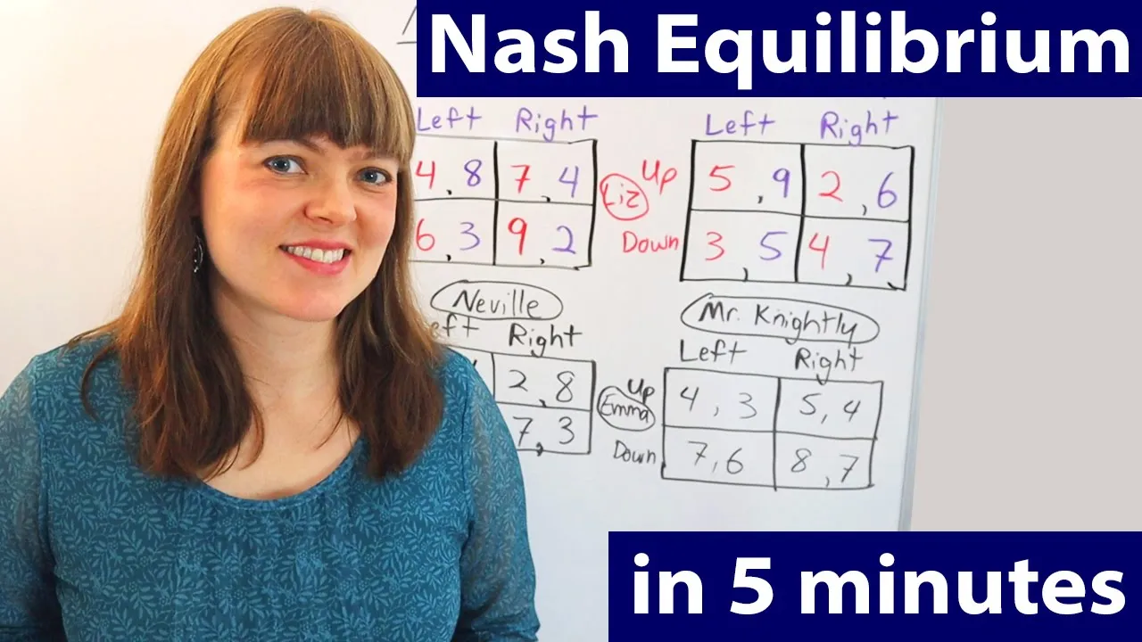
Basic game theory concepts, particularly the definition and derivation of a Nash Equilibrium in simultaneous-move games.
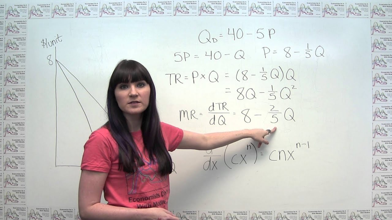
The algebraic and graphical representation of demand curves, total revenue, marginal revenue, and cost structures.
Standard profit-maximization principles, including how firms set quantity or price to maximize profit.
The Stackelberg model of oligopoly, exploring the strategic dynamics and first-mover advantages of sequential-move quantity competition.
The Bertrand Paradox and its resolutions, including Bertrand competition with capacity constraints (Edgeworth model) and product differentiation.
Collusion, cartel behavior, and tacit coordination, studying how repeated games can sustain cooperation and high prices over time.
Antitrust economics and merger analysis, learning how competition authorities use oligopoly models to evaluate market power and consumer welfare.
129.6K views1.7Klikes11:07Original Release: 2010-08-30
In this video, I'm going to give a survey of the two big competing ideas about how to think about oligopoly. On one hand, we have Bertran competition and on the other hand, we have corno competition. I'm going to give a survey of the intuition. What key terms should pop into your mind when you think about these two types of competition? And then I'm going to give a sense for the mechanics. How can you work a problem that deals with Bertrand competition?
How can you work a problem that deals with Corno competition? So let's start with the intuition and we'll compare Bertrand and Corno. So Bertran competition is competition on price. A word that should pop into your mind when you think about Bertrand competition is the incentive to undercut. You should think that this is very vigorous competition. It's very vicious and you shouldn't think that there are much profits to be made when you are competing on price because competing on price as we'll see in the mechanics section is going to drive profits all the way. Now in contrast corno competition is competition on quantity.
Sort of the way it works is that each firm picks a capacity to produce at and then just sees what price prevails in the market. Now compared to Bertrand competition, corno competition is much nicer. It's more of a give and take. And yes, there are going to be profits left over from corno competition. So you might not mind being in corno competition. So let's consider what happens as far as the mechanics. We've got an inverse demand curve of P= 30 minus Q. We've got a marginal cost of zero. Now, inertran competition the way it mechanically works is say we have two firms uh in the market. Each gets to pick a price and they pick simultaneously. But if they pick wrong and they pick the the higher price, they get no customers because all customers go to the lowerric product. Therefore, think about a firm that's considering setting a price of, let's say, $10. If firm one decides to set a price of $10, they're really going to be worried that the other firm is going to undercut them by setting it at $9.99 and it's not stable because they know that the best response to a price of $10 is going to be undercut by uh by some amount. If they set a price of a dollar, the other firm will set a price below that and so on and so forth. And so what you'll see is that there's always going to be this worry that you're going to be undercut by your competitor. And so you're never going to pick a price that's above marginal cost. If you pick the price equal to marginal cost, what you'll notice is that if uh if your competitor undercuts you, that's going to be to your competitor's detriment because they'll make a negative profit in that case. And so only when there's no longer an incentive to undercut do the firms stop undercutting each other sort of in their in their mind. So or stop worrying about being undercut. And so the only price that can actually come about here is price equals marginal cost.
So in this case we would set the inverse demand curve equal to the marginal cost of zero and that would give us our uh that would give us our quantity the the total quantity that would be sold in this market and then because they set the same price in equilibrium what we'll end up with is we'll end up with them splitting the market each producing 15 at a price of zero in this case. You can see this is very vicious competition.
We get a price of zero and neither firm makes any profits. So that's that's a really bad situation. And that's really all you need to know about the mechanics of upper trend competition. Set price equal to marginal cost. And it sort of emulates what we had back in perfect competition but for a different reason.
These are price setting firms that are responding strategically to one another.
and their best response is to keep decreasing their price until it equals marginal cost. Now, let's move on to the mechanics of Corno. And these are a little bit more involved, but they rely, as I said or hinted before, on monopoly mechanics. So, let's let's consider this particular example. We're going to think that there are going to be two firms in this industry. So, this big Q is going to be the sum of those two quantities.
Now look at this from the perspective of firm one. Firm one can only control quantity one. That's the only part that goes into the slope of the demand curve that he really effectively faces. So what we can do is we can reshuffle terms. So all I did is I moved the term involving Q2 over by the intercept and I left Q1 over here where we're going to think of that as slope times quantity.
Now firm one can't control this part.
So with that in mind, what we can think of is that this to get our marginal revenue for no competing firm, what we do is we take the intercept and twice the slope. This is the intercept. We take twice this slope. So here's our marginal revenue. Notice that now because the other firm spped up some of that demand, what we get is we get a marginal revenue that depends on the production that the other firm uh uh how much the other firm produces. But that's all right. We can we can go and work with that and just say let's set marginal revenue equal to marginal cost.
And remember when we're setting marginal revenue equal to marginal cost, we're picking the quantity Q1 that maximizes profit. So if we solve this equation 30 - q2 - 2 q1 = 0 for q1, we'll get what we consider to be the optimal response for firm 1.
Now this function here is what would call the best response function or the reaction function. And it tells us the best quantity that firm one can pick given a choice that firm two picks. And what's interesting about this is that if firm two produces more, the best response of firm one is to produce a little bit less. Or alternatively, if firm two produces less, the best response of firm one is to produce more.
So there's sort of a give and take nature to the strategy of firm one given what firm two does. And their strategy is how much quantity do I produce. So this is very different than the strategy over here in Bertrand where if I decrease my price, your incentive is to decrease your price. This is uh we're giving and taking. We both and incentive to raise the price. And we're doing so sort of in a nice way that doesn't compete all the profits away. So what we can do is we could do a similar exercise for firm 2. We would get a symmetric equation here where this would be Q2* = 15 - 12 Q1 because everything is symmetric in this in this example. And then if we want to solve for the quantities, we would just have this equation and the one that we uh we got from for firm 2. And we would solve those two equations and two unknowns because it's symmetric. Q1 star and Q2 are going to be the same. And so we could use some symmetry in this to actually solve what the what the ultimate answer is going to be. Q1 equals 10 in this example or in total Q1 plus Q2 because they're both equal to 10 that's 20. If we plug back into the demand curve we get a price of 10. Now notice the price is higher. We're actually going to make some profits in this example. And so you can see that uh once we do the full-blown coro competition that we end up getting more profits wi under under coro competition than we do under bertrand competition wi without uh sort of pushing the envelope too much farther. What we can do is we can extend the coro intuition into a leader and follower game that takes place over time. So when we do this and we say uh we have an individual who gets to move first or a firm that gets to gets to make its capacity choice first uh and then a follower who has to respond to that capacity choice and has to take that into account. That's what's called stackleberg competition. First mover in the stackleberg game can reason through what firm two is going to do in response to his capacity choice because he can reason through what firm two is going to do in response to him. He can sort of anticipate uh what quantity firm two is going to going to pick and more than just anticipate by picking his capacity.
It can dictate what firm two is going to do. So there's not going to be any uncertainty about what's going to happen. So firm one will put himself in the shoes of firm two. Reason through that firm two is going to respond via a corno style reaction function. And then when you reason through it, what you'll see is that if firm one produces more, firm two will want to produce less. That means that firm one will want to produce even more, which means firm two will want to produce less. This will eventually sort of sort itself out and settle down. But what ends up happening is that if you get to move first in a stackleberg game, you get to uh expand, take more of the market and leave less for the corno competitor who gets to come later because you get to set your capacity first. You get to dictate to the follower that they have to take a smaller quantity that remains. And so you can end up getting a first mover advantage in that in that case. And that comes from this cowering effect. I produce more. That means that you'll want to produce less. So that's uh that's the the basics of oligopoly. Some bertrand, you have corno. If you want more details, I go into more details about bird when you have multiple uh multiple products in in lecture 35A.
And in lecture 35, I've go over corno but with uh with some calculus as well.
I go through an entire example demonstrating how to do how to do a corno example.
Up Next
18:01
Cournot Oligopoly: Equilibrium vs Monopoly & Perfect Competition
@kfhinde
143.3K views•2011-11-15

5:07
Impact of Yuan in Indo-Russian Trade Amid Sanctions
@WION
261.9K views•2022-07-01
10:33
Behavioral Economics Explained: Rationality, Nudges, and Risk
@crashcourse
1.1M views•2016-03-12

113:18
The Age of Easy Money: Fed & Inflation | Full Documentary
@frontline
21.2M views•2023-03-15
Related Study Plans & Knowledge Roadmaps
Structured learning paths in Economics
economics
Sovereign Debt: Defaults, IMF & Restructuring
01Introduction to Sovereign Debt & Government Bonds
02Debt Sustainability & Credit Ratings
03Anatomy and History of Debt Crises
+ 2 more learning modules
12h5 modules
Explore Roadmap
economics
Market Design: Matching Theory & Gale-Shapley
01Introduction to Market Design and Price-Free Markets
02Two-Sided Matching & The Gale-Shapley Algorithm
03School Choice Systems and Mechanism Design
+ 2 more learning modules
10h5 modules
Explore Roadmap
economics
Impossible Trinity: Forex, Capital & Policy
01Introduction to Monetary Policy and Central Banking
02Exchange Rates and International Capital Flows
03The Mundell-Fleming Model
+ 2 more learning modules
8h5 modules
Explore Roadmap
economics
Healthcare Economics: Market Failures & Systems
01Introduction to Healthcare Markets and Market Failure
02Asymmetric Information and Adverse Selection
03Moral Hazard and Insurance Design
+ 2 more learning modules
12h5 modules
Explore Roadmap