














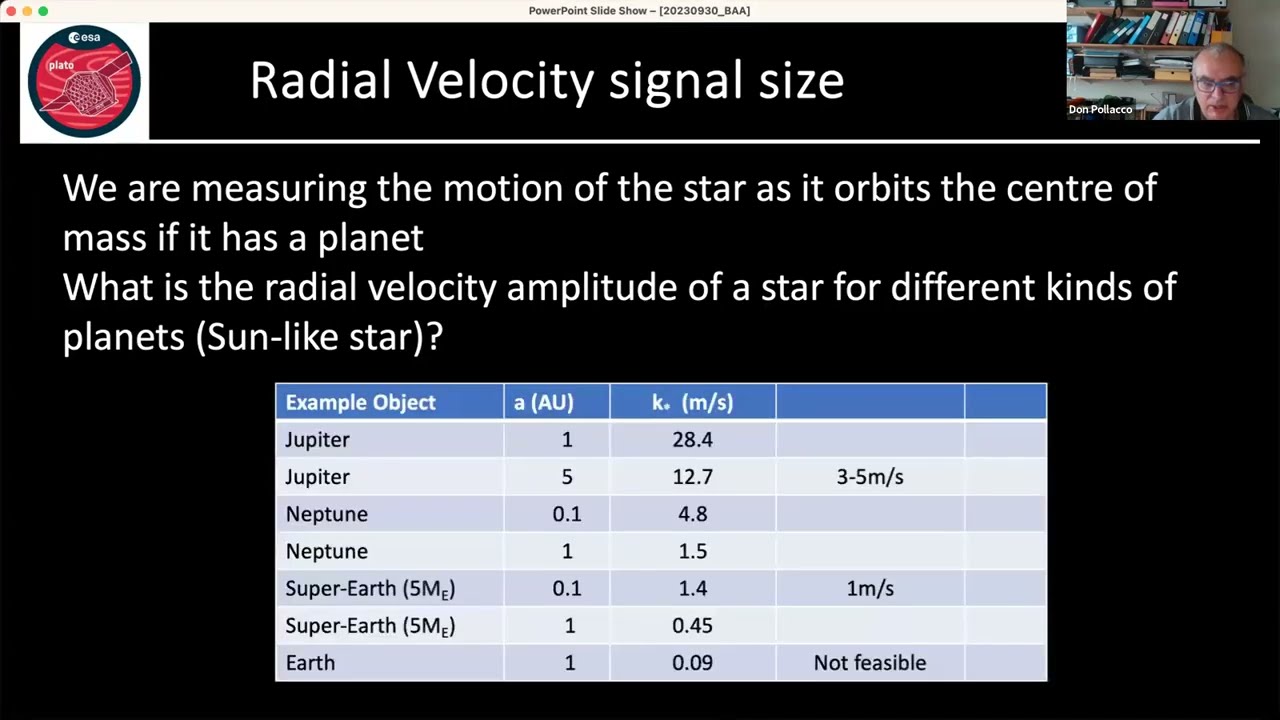

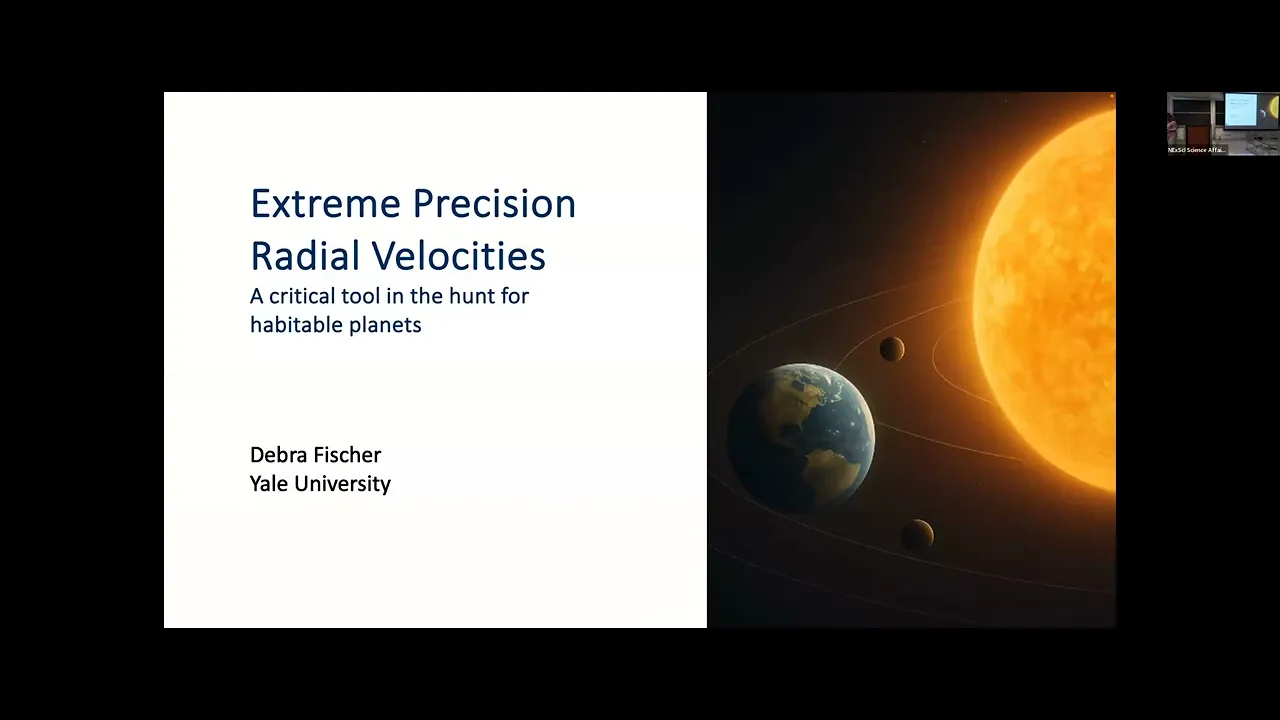







The radial velocity method detects exoplanets by measuring the Doppler shift of a star's light, revealing reflex motion caused by gravitational tugging from orbiting planets; the resulting RV signal amplitude (K) depends on the planet's mass, orbital period, stellar mass, and orbital inclination, with the formula K = (2πG^(1/3)M_p^(2/3))/(P^(1/3)(M_*)^(1/3)) × sin(I), where the sin(I) term means RV measurements only provide minimum planet masses rather than true masses.
Deriving the Radial Velocity Equation | Exoplanet Detection Series
Added:Kepler's Laws of Planetary Motion and the concept of a barycenter (common center of mass) in binary systems.
Newtonian Mechanics, specifically centripetal force and the law of universal gravitation.
The Doppler Effect and how relative motion affects the observed wavelength of electromagnetic radiation.
Basic trigonometry and vector projection, particularly projecting 3D orbital velocity onto a 1D line of sight using the inclination angle.
Calculating the minimum mass of an exoplanet (m sin i) and understanding why the inclination degeneracy prevents determining the true mass.
Analyzing real-world radial velocity curves and fitting Keplerian orbits to noisy data affected by stellar activity (jitter).
Combining radial velocity measurements with transit photometry to determine an exoplanet's true mass, radius, and bulk density.
Exploring advanced spectrograph technologies and calibration techniques, such as laser frequency combs, required to achieve extreme precision in astronomical observations.
3.3K views165likes11:41Original Release: 2020-07-08
Welcome to chapter two in the exoplanet detection series here in the Cool Worlds Classroom. In chapter one, we established some foundational results in celestial mechanics and that meant a lot of mathematics, a lot of hard work, but now we get to reap the rewards of all of that effort. In today's video, we will be using those earlier results to derive the equation governing the radial velocity method of detecting exoplanets. Radial velocity detections dominated planet catalogues for the first decade and a half of the exoplanet era and are often still considered the gold standard of planet detection. For these reasons then, it is crucial for every exoplaneteer to understand how this method works.
There's a lot to be said about the radial velocity method, far more than I am able to cover in a single short video. Now as discussed in the trailer for this channel, the videos that we have posted so far are really just a sample set and we're hoping to find funding to support the content here going forward into the future and, in that vein, this video today will actually be the last video of this sample series. So if you haven't already then please do offer us some feedback so that we can make these videos even better going forward into the future.
Back to the topic at hand, you might be wondering who is pictured here at the bottom - this is Otto Struve, an astronomer often credited as the first person to consider the possibility of detecting exoplanets with the radial velocity method all the way back in 1952. His short essay didn't get noticed much until recent years but I think it's a remarkable historical example of scientific foresight. Now the basic idea of the radial velocity method is likely something that you've encountered before, but it's very simply the act of measuring the red or blue shift of a star's light, or more precisely a star's spectrum. These red and blue shifts tell us how fast the star is moving relative to the Earth - its velocity. After correcting for the Earth's orbital motion any changes in a star's velocity means an acceleration, dv/dt, and we know from F=ma that whenever there's an acceleration that means there must be a force responsible.
Now when it comes to moving a star, really the only force that's possible here is gravity, and so immediately just seeing a change in the radial velocity tells us that must be a gravitational body, such as a planet, nearby tugging on that star. Here, we see a snapshot of a star moving towards us in response to its planet. This is often dubbed reflex motion. In this snapshot, the star is moving towards us and so it would appear blue shifted. Now recall from video 1D that we define the observer to lie along the Z axis, since radial velocity exclusively refers to motion along the line of sight then that means that we are measuring dZ/dt. OK, now also from video 1D, we obtained these Cartesian orbital elements. The top here is the heliocentric planet positions and the bottom show the planet and stellar motion in the barycentric frame of reference. So that Z* term over here is the one that we really care about.
Specifically, a radial velocity is conventionally defined as -dZ/dt plus a constant, gamma, which is just the speed at which the star is essentially drifting through the galaxy. The choice of that minus sign is just by convention, it's totally arbitrary, but it means that things moving away from us, which are redshifted, have a positive rate of velocity. Let's save these two equations and move them over to a new slide. That r term in the Z* equation represents the planet star separation and is something that we determined back in video 1C, so let's just plug that in. That yields the following, which can be tidied up a little through rearrangement to this. Now let's go back to the RV equation and expand it using the chain rule, this helps us because we can't directly differentiate Z with respect to time but we can do so with respect to true anomaly, f. The df/dt term is again something that we derived earlier in video 1E, so we cannot just use that result here. After differentiating, you should be able to show this result for the RV signal, where K is a time invariable quantity known as the semi amplitude given by this. Now I want you to pause the video here and try deriving this for yourself - to do that differentiation and rearrangement step.
Make sure that you get the same result. All right good job. Now let's see what these RV signals really look like. Here's a pretty famous example, it's our nearest star Proxima Centauri, which has an Earth-mass planet around it. Here we have a nice circular orbit giving us a sinusoidal signal, but we'll later show how eccentric planets can look quite different. So the semi amplitude K can really just be read off this plot. So too can the orbital period P given by the time it takes for the signal to repeat itself. The RV function is this red line, which has actually been fitted to the data given by the teal points. So already we can see there's a lot of information about the planet encoded within this data set. If we look at this equation for K, we see both a, the semi-major axis, and P, the orbital period, featuring. But via Kepler's Third Law, that is generally redundant, so let's replace a with P, since P is the only observable between those two. Why? Well, remember that I can read P off that plot back there but I can't read a off that graph, there's just nothing directly telling me what the semi-major axis is. After replacing with Kepler's Third Law, this gives us the following more conventional way of writing the semi amplitude equation.
Another way of writing this is in so-called canonical units, where we plug in numbers for a fiducial example. In this case, a Jupiter on a one-year period around a Sun-like star, and then we rewrite the parameters as scalings.
This is instructive because it gives us a sense as to how big the signal is and the relevant proportionalities. Note that I have also assumed here that mass of the star is much greater than mass of the planet, just to simplify things a little bit. So let's look at these scalings closely. The RV semi amplitude K decreases with P, but not very steeply, just with a 1/3 power.
So what that means, for example, is that a planet with an 8 times longer orbital period would only reduce the semi amplitude by a factor of 2. Turning to M*, we see an almost inverse relationship which means that lighter stars give bigger signals. OK that makes sense, because lighter stars are easier to wobble and finally we find a linear scaling with respect to planet mass - that means that heavier planets wobble the star more and are thus easier to find.
Critically, notice that there's a pesky sin(I) term in here. That sin(I) term is crucial because, in general, we don't know what its value is.
So in truth, we don't really measure Mp - only Mp multiplied by sin(I). Now since sin(I) is a number which is always less than 1, then that means that Mp sin(I) is often referred to as the minimum mass. This is a really important and basic limitation of the radial velocity method. Truthfully, radio velocities don't measure planet masses, they only measure minimum planet masses. If we go back to the full equation, without assuming M* is much greater than Mp, I want to highlight another important point. These terms here are easily known - there's G and pi, which are just constants, and P which comes from the periodicity of the RV signal itself. Likewise eccentricity can be measured from the shape of the RV waveform. But this stuff here in the middle, this is a-priori unknown and directly controls the semi amplitude. It's a bit of a mathematical jumble, and is often just simply coined the mass function, or to really follow historical convention it should be called the cube of the mass function. Now the problem with this mass function is that Mp, the mass of the planet, appears in two places. It's non trivial to rearrange this equation and get Mp equals something - in other words it's tricky to figure out what a planet's mass is for any given RV signal. Now there are strategies to do this. First, as we did so earlier, we can just assume that the star is much heavier than the planet essentially ignoring the Mp term in the denominator.
That makes the math far simpler. We can now directly solve and that's actually the most common practice, but it is of course an approximation and thus not entirely correct. The second, and more challenging approach, is to solve the cubic equation in Mp, which can actually be done analytically, although it's rather ugly. How different are these two results? Well for the heaviest of planets, or even brown dwarfs, the tension between these two could perhaps become significant, but actually I don't know how significant. So why not investigate this for yourself as a mini research project? Try calculating the mass of the planet from K, P and e as listed in the exoplanets.org catalog using these two methods for a bunch of planets and see whether they disagree by more than the formal errors. As I said, I don't know the answer to this - this is genuinely a novel research idea so please go ahead take it and have some fun.
So that wraps us up for today and indeed for this sample set of videos. Now obviously there's a lot more I could and would like to say about radial velocity so hopefully we'll get funding to extend this series in the future, and if we do we'll be able to talk about not just other exoplanets detection methods aside from radial velocities but even entire new series besides from the exoplanet detection series as well. So if you have any feedback about the videos we've produced so far, I mean this is a sample set so this is the time to give us some direct feedback, let us know what you think and how we could maybe improve it going forward. Thank you so much for your time and watching these, if you are missing us in the meantime before we come back then do make sure you check out our main channel over at the Cool Worlds Lab - until then bye for now.
you
Up Next

49:59
Doppler Effect, Binary Stars, Neutron Stars & Black Holes | 8.01x Lecture 23
@lecturesbywalterlewin.they9259
134.5K views•2015-02-08

12:53
21cm Hyperfine Transition in Neutral Hydrogen: Radio Astronomy Basics
@AaronRobertParsons
12.4K views•2011-10-13

32:32
NMR Spin Physics I: Zeeman Effect, Resonance Condition & Larmor Frequency
@nptel-indianinstituteofsci8064
2.3K views•2024-01-17

27:14
Entropy and the Second Law of Thermodynamics Explained
@veritasium
27.5M views•2023-07-01
Related Study Plans & Knowledge Roadmaps
Structured learning paths in Physics
physics
Nuclear Physics (Decay, Fission & Reactors)
01Atomic Structure and the Binding Force
02Radioactive Decay and Half-Life
03Nuclear Fission Mechanics and Chain Reactions
+ 2 more learning modules
12h5 modules
Explore Roadmap
physics
Soft Matter (Polymers, Colloids & Rheology)
01Foundations of Soft Matter & Thermal Forces
02Polymer Physics and Macromolecules
03Colloids, Surfactants, and Self-Assembly
+ 2 more learning modules
38h5 modules
Explore Roadmap
physics
Analytical Mechanics: Lagrangian & Hamiltonian
01Mathematical Foundations: Calculus of Variations
02From Newtonian Mechanics to Constraint Dynamics
03The Principle of Least Action & Lagrangian Mechanics
+ 3 more learning modules
28h6 modules
Explore Roadmap
physics
General Relativity (Spacetime & Cosmology)
01Foundations of Relativity: Special Relativity
02The Geometry of Spacetime: Equivalence Principle & Curvature
03Einstein's Field Equations: The Mathematics of Gravity
+ 2 more learning modules
55h5 modules
Explore Roadmap