Fluid Flow Instability and Transition | Aerospace Engineering Lecture 1

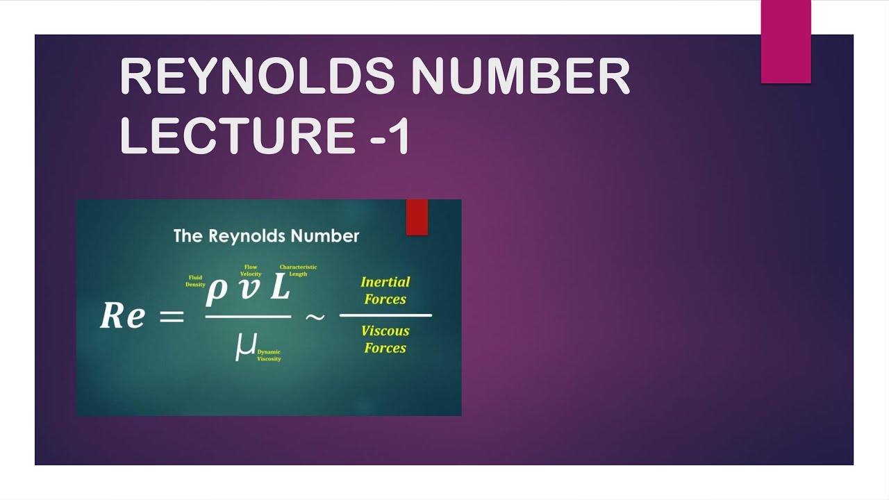
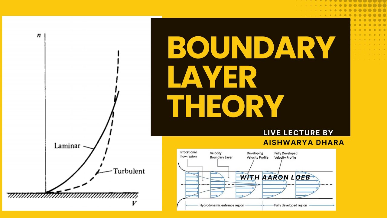
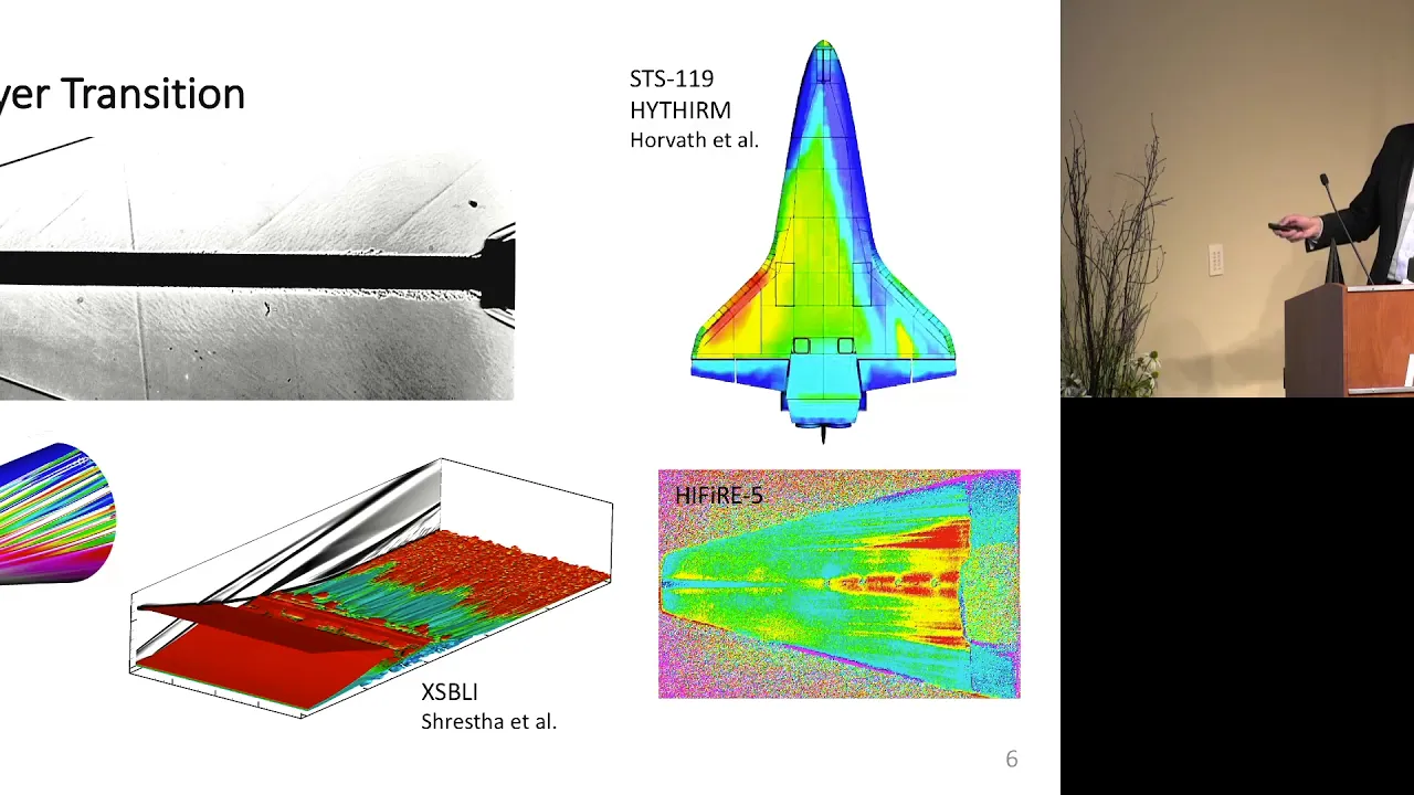
[00:00:16]ah good morning uh welcome to this course on transition and turbulence a625 uh you can get my name and affiliation contacts are given here i would prefer for that you can come anytime that you wish to and just give me a phone call and just walk in the title itself would uh suggest that we are looking at fluid flow transition uh the instabilities that lead the flow to turbulent state that's what is the main theme of this course ah as we begin today let me try to tell you a little bit about the scope of the course the contents uh we'll start off with the introduction on instability and transition that's what we'll begin today itself we need to really look at how the way the subject has developed over the period it was quite early on understood that actual fluid flow behavior depends on flow instability that means what that you have governing equations of motions and those equations of motions are most of the time non-linear partial differential equations are not solvable uh in some specific cases you could solve them and once you solve them you would notice that that you you get some analytic solution and you go to the lab perform the experiment and you do not see them that is exactly what happened to strokes so gigi stokes who is associated with the development of navier stokes equation so he solved flow passed inside a pipe and tried to compare his analytical solution with experimental data and he did not find anything so it does mean that not all solutions are observable we can see them so this is one thing that has really triggered the attention of many people so that is what we want to study in instability of in fluid mechanics because this is related to the instability of the solutions what is instability that if i have a solution or if i have a physical scenario then if i also have some background disturbances which is not in my control they do affect and instability implies those small imperceptible disturbances to create large effects that's what we mean by instability small cause leads to large disturbances and there are classical theories developed and you would be quite amazed if you have not heard of it before that it was one of the pioneer in physics who actually picked this problem up to solve and he is no other than heisenberg as a student of summerfield he first started looking at flow instability and subsequently the german school led by prandtl and his students actually started looking at it ah two notable students are tallman and schlichting those of you have seen the book by schlistering so this is the same gentleman they worked on it and what they found that the flow becomes unstable and then you also see some waves so this is what we mean by ah this is what you mean by heisenberg tolmenschlistein waves that we have written there will will be spending quite a bit of time talking about that what is important to realize that again those theoretical prediction of instability theories are not to be seen in experiment so you can see that as a engineer by training or as a scientist by training you cannot compartmentalize your activity you cannot just simply say i am a theoretician i do not know i don't care about experiments the same way experimentalist cannot make that same claim that we do experiments if we don't see it then your theory is wrong this happens all the time it's unfortunate business and to tell you in this context also similar thing happened when this uh three people of one after the other started predicting these waves it was nobody else other than pressure g.i taylor of cambridge he tried to experiment and when he tried to perform those experiments he did not see those waves and so that led to a sort of a very big debate international debate the german school is saying that there are waves and the english school led by j i teller says there are no waves so what happens that is what is a big story then came into the picture is this group from usa dryden and his colleagues two of his colleagues shubar and scramstadt did perform some classic experiments at national bureau standard in washington they did those experiments and they were the first to observe those waves and to perform those experiments that work very hard they realize that not all kinds of disturbances give rise to waves so as a mathematician always you would see like people talk about flow instability in terms of eigen value problem so eigen value problem is what you have a homogeneous equation homogeneous boundary condition and you try to get a solution out of it and those are your eigen solutions so what does it mean actually it means as if something is falling from the heaven you are not putting any effort and you are seeing some results right so that's another drawback of eigen value analysis what one should instead look at is connect the cause with the effect so cause will be those background disturbances they may not be always measurable but they still would have some quality and that is what shubar and scramstadt found out shubha and scramstad noted that not all disturbances produce waves they could produce waves only when they vibrated a ribbon inside the boundary layer they found out that if you try to excite the flow with acoustic noise it does not create waves and that is the subject that we talk about in this what we call as receptivity that the flow is receptive to certain class of disturbances not all disturbances can give you instability waves ok so if we are going to do that we need to actually instead of studying stability we should be studying receptivity and that is a major thrust in this course perhaps unique in all over the world that this subject is addressed in that framework we do it here so we will be talking about receptivity and what we would also notice that this experiment that was done by shubha and scramstad required extreme care in setting this experiment up you have to create a virtually noise free background reduce the disturbance as far as possible so they actually designed a very very nice wind tunnel that wind tunnel even 70 years afterwards continued to be used somewhere in some u.s universities so you have to design an internal you would find that there would be many experimental facilities they make unsubstantiated claim that we have a very noise free tunnel but they have no measurement of noise though well we will not talk about that ah what we are going to talk about is the reality not the virtual one where people make tall claims you really have to design a tunnel where background disturbances have brought down to zero and then only you have to excite the flow deterministically like as i told you in shubar's gram start experiment that inside the boundary layer you started vibrating a river what happens if the amplitude of that vibration becomes very large you don't see those waves you don't see those waves so what happens is any transition any instability and transition that takes the flow from a laminar state to turbulent state without showing the waves have been historically called in the literature as bypass transition so it bypasses the root of that heisenberg tolman schistic waves right this is what we would be studying then people also have realized that there are a large number of cases where your stability analysis shows the flow to be unstable but in reality those flow also become turbulent there are no flows which remain laminar forever so please do understand that laminar flow is an exception turbulent flow is a rule ok unfortunately bias in all the programs is to pretend as if laminar flow is everything and turbulent flow is a specialization it is not true people should know turbulent flow more than they should know about laminar flows ah but to even to know how the turbulent state appears you need to know this process of transition from laminar to trouble that is precisely what we are doing in this course right ah what happens is as i told you that there are many flow situations where you would not see these waves it is bypassed etcetera and there are also cases where the instability theory even says that it should not become unstable and nothing more to exemplify this is the case of a let us say pi flow theoretically it is shown to be stable but we all know that reynolds number above 2000 based on diameter of the pipe flow becomes turbulent then there is a squared flow shear driven right if i have flow between two parallel plates and the top plate is moving that is what we call as a weight flow quit flow is also theoretically found to be stable right however those flows are not really stable so people have tried to study one of the mechanism people talk about is some kind of a special temporal instabilities um that may be affecting some of these flows and this is what we are trying to look at okay ah this is about wall bounded flows external flows that we have been talking about because most of us have a background of aerospace engineering so we are more more interested in external flows but then we also at times have to worry about not streamline shape we have to worry about bluff shape think of an aircraft when the landing gear comes out that's a flow past a cylinder right ah well there are many many such occasions you would see there are cavities etc so there what happens is we do not have streamlined body flows instead we have blood body flows and they also suffer some kind of an instability ok now instability per se instability per se can also occur in two different ways or a combination of these two ways what are these two ways the disturbances can grow in space disturbances can grow in time and disturbance can also grow in space and time that's what we talked about special temporal instability disturbances which simultaneously grow in space and time now this earlier part external flows that we talked about past streamlined bodies one of the characteristic feature people have noticed over the years is that there the disturbances actually convect as they grow that means it's a spatial growth growth in space okay in contrast to that let us say flow past a cylinder is looked at a blood body flow there you notice that initially the distances grow in time if you are positioned in the wake you look at it you will see it grows in time now it is an interesting thing that that is a that is a basically a sort of evidence of instability the disturbances are growing but non-linearity plays a very different role for this external flows of past streamlined body and a blood body for a streamlined body what happens the nonlinearity actually accentuates increases the instability that's where you go please do not understand make this misconception that flow becomes unstable and boom it becomes troubling it doesn't happen that way the instabilities grow then that disturbed flow further can become unstable so the first instability will call it as a primary instability the subsequent ones will call it as secondary instability tertiary instability and so on and so forth so for a streamlined body flows the primary instabilities are predicted very nicely by those classical theories while the secondary and tertiary instabilities are due to some kind of non-linear effects and they actually accentuate the instability while for a flow positive body will show that the primary instability is a temporal instability and non-linearity here plays a very interesting role non-linearity here actually modulates moderates the primary instability so the waves keeps growing but then it saturates ok we will see this will spend lot of time doing this so these are some of the interesting things that we would be talking about and you have heard of landau landau came out with a equation which is called stewart landau equation that tells you how this primary instability saturates into a non-linear action into another almost neutral amplified waves so you start off from one equilibrium state that was your laminar flow it became unstable because of temporal instability the nonlinearity saturates it so you actually get a time periodic flow this is what you see as the vortex shedding behind the cylinder that is a classic example that you have a vortex shading carbon ah bernard vortex shedding behind the cylinder you say that they are very periodic they do not just simply explode that happens due to this non-linear action and lambda actually worked out the equation for it and will also talk about bifurcation what is bifurcation now we are talking about instability of flows as i told you flow inside a pipe the classical linear theory says its stable but if i perform experiment i find that flow cannot be kept easily laminar if the reynolds number is above 2000 if it is above 2000 then you will have to make some effort additional effort to keep the flow laminar but if your reynolds numbers are less than 2000 then even if you create a lot of disturbance in that flow it still remains laminar so it seems the reynolds number works like a kind of a parameter for the problem and you have a critical value below which it remains stable above which it is unstable so this kind of a scenario where actually we may look at ah let us say flow past stage cylinder if i were to be talking about on this axis i will be plotting say reynolds number based on the diameter and on this side let me just simply ah plot the amplitude so basically what we are talking about that ah um we are going to get some disturbances ok so this let me write it as ud subscript d implying disturbance field and that i will write it as some a of t i told you it suffers from a temporal instability so let us call that as a of t and that would be multiplied by some function of space f of x right now this is that a that we are plotting the time dependent thing what we find that up to some reynolds number that up to that the flow remains laminar that means what this amplitude does not right so you even if you create some disturbance that disturbance will eventually decay so this is something like your equilibrium flow ok what do you mean by this so what we can do is if i plot a of t versus t i may get something like this that initially let us say i create some kind of a disturbance and if i am below this r e critical critical value then what will happen it may just simply go and go and decay that is sub critical flow right so this is the sub critical part ok and this part i will call it as super critical so this is your a sub critical solution where you may have initially created some disturbances at t equal to 0 but eventually decays whereas in case of a supercritical case what happens is something different happens there what we will find that suppose i start off with some virtually no disturbance at all but there are background disturbances in the experimental facility then what will happen for a super critical scenario i would have something like this i will show you detailed results of this theoretical computational as well as experimental people have done it and they really find that something very interesting thing happen it remains virtually like this then you actually see some kind of a very high frequency oscillations ah once in a while and then it slowly picks up so this is what we meant by ah blood body flow instability and then what happens is it just saturates to in an envelope and this growth of the amplitude curve is what is of interest so in the super critical case what happens is you are going to see that starting from r critical this is your equilibrium state so this is my ae that we are talking about this is that ae the amplitude it is two times right it is a periodic oscillation so it is two times a so i can plot that and what you would find that the scenario is like this that up to recretical that equilibrium amplitude remains zero and then it actually goes like this so this behavior is typical of blood body flows and this transition from a subcritical to super critical state is what is often called as bifurcation now why why do we call the solution bifurcation it means that in the supercritical stage i can actually get a solution which could be here or if i am carefully doing the experiment i can also assume to have this case for example for the pipe flow experiment we will talk about today itself time permitting osborne reynolds did those experiments we talked about just now a reynolds number of 2000 being the critical reynolds number osbourne and alzheimer carefully did those experiments and he could keep the flow laminar all the way up to 12 830 okay nothing to be surprised about because later on people even did experiments and created pi flow which are stable for renault's number hundred thousand so what it means that your solution bifurcates from this point onwards here you will only have one solution but here you will have multiplicity of solutions ok wow this is a very very uh typical attribute of systems which suffer temporal instabilities ah specially flow past blood bodies you can think about so this kind of bifurcation is what is called as a hop bifurcation well there are many types of bifurcation hop bifurcation is one of it so will will use that and we will also talk about other interesting things like effect of heat transfer around flow instabilities this is a very very important issue because if we are talking about let us say flow past flow in our atmosphere the weather system here what you have you cannot just simply talk about the instability of the atmosphere only in the absence of heat transfer the heat transfer as it occurs sun is our main source of energy but we these days we are also creating lot of uh heat ourselves right anthropogenic heat transfer right man-made heat how does it affect the system dynamics you got to understand that in this course we are going to take a very very deterministic approach of systems in studying their instability so what we are going to talk about is basically a system which i would represent by a let us say black box so this is your system right now what happens to the system this system is bombarded by input we like it or not they are there that is what we have been studying right and then we get an output and we have already seen the talking about receptivity is basically trying to connect input with the output through the system dynamics what is the system dynamics ok for the time being i will call that as the function so what does this system do it takes the input multiplies it by the transfer function to give you an output transfer function is done the property of the system so i can have flow pa in the weather system ah without those heat transfer i am talking about one kind of transfer function the moment i add the heat transfer the transfer function has changed this is what i was telling you also about reynolds experiment he did something to change the transfer function or he did something to reduce the input right so there are lots of very very interesting thing in studying any dynamical system this is basically is one of the goal of this course that we talk about systems in nature as a dynamical system talk about the economics of a country its a dynamical system right we do not know how to model it we cannot get its transfer function correctly that is a different issue but hopefully in future we should be able to do that look at all those smart alecks in the finance field they actually play around find out how this micro fluctuations in the input and they convert it into dollars in their pocket right that's also they study they use chaos dynamics right so we talk about this any practical system tells you that this transfer function need not always be very deterministic a very good example is as i always am fond of coating is tossing a coin we cannot even predict its transfer function why ah i mean that's a part philosophic part physical but the fact is we do not know what are the players that determine the outcome right ah the same way economics as a subject we do not know there are too many contributing factors that makes the study of that dynamical system very very difficult you cannot get a deterministic portrait of it we have to talk about it as a stochastic system and that happens this stochastic system means what it's probabilistic but also time dependent that is stochastic right tossing a coin could be a probabilistic event but we don't know whether it is stochastic or not because if i am doing the experiment in this room tossing a coin ah depending on how the temperature inside the room is changing with time etc or if i keep a windows open or something and the head drifts in that can all affect the outcome of the experiment so whether it is simple probabilistic time independent or it is time dependent that is stochastic we do not know so basically um in terms of instabilities as affected by heat transfer is a worthy subject that gives us a some glimpse of what may happen to a complex system we will be talking about that and then i will talk about secondary and three-dimensional instabilities back to our aerospace applications where we will see how this secondary and the three dimensional instabilities come into play and i told you very clearly about this aspect instabilities and transition instability does not mean that you would get a transition immediately right so basically instability and transition are not synonymous you have a finite region over which the flow becomes unstable so if i am studying a flow past aerofoil so the flow can become critical at this stage but if i am looking at say fully turbulent state it may have happened here so this is what i may call as a critical point and this is where let us say finally the transition takes place well there are various definitions of transition quantifiable so let us say we adopt one of those and that says it is there so this is a very non-trivial space so this is what we will be calling it as the transitional flow so on this side we have laminar flow and on this side we have turbulent flow and this two are bridged by transitional flow right so it so happens that this region over which transition occurs is not trivial a very good example would be a flow in a turbine and a gas turbine you know in a turbine flow accelerates accelerate means it is under the influence of favorable pressure gradient while that turbine also sits downstream of the combustion chamber and combustion through those all this chemical reaction makes the flow very very dirty very very noisy so you have a competing dialogue going on you have a dirty flow coming in bombarding and you are imposing a acceleration which is trying to moderate that makes this region very very significantly large so to understand transitional flow is a very very important issue and that is what we need to really keep aware of and once you come to the turbulent state you need to know what is really turbulent flow and i would type permitting i will talk about this morphology what constitutes in this course we are not doing turbulence modeling i mean we we we would keep that aside we will focus on the scientific aspect of it we will talk about it see ah basically all we want to do eventually try to understand what turbulent flow so we have taken a different route now to in understanding this we are coming from the laminar flow side and see where we are our point of view is that the turbulent state where we arrive would be determined by the process of transition it is not unique ok now we have seen what our course of content is going to be like this this is something you must be also curious to know what are the references that we are going to use well we are going to use this book this is a book that myself and ah dr point so i have written uh will not do the chemical reaction part we'll just do this part instability of flows with and without heat transfer right so this book is available apart from that book i would recommend that one looks at this book by drazen and reid it's now quite a classic book titled hydrodynamic stability and this two will be more than adequate there are many other books you can take a look at them but it's not necessary okay so we'll stick to this two books only and that should be adequate and in the turbulent flow part we have a very nice book here first course in turbulence by tennicus and lumley that is one book that we would be using in bits and pieces ah but for understanding the morphology of turbulent flow we would also be looking at this applied analysis of the navier-stokes equation by during and gibbon ah this is a very short monograph but very nice book nice book and as we seen and discussed that we like to study the flow as a dynamical system and we try to find out what its transfer function etc is so that is covered very nicely in this book uh called turbulence coherent structure dynamical systems and symmetry for holmes and lumley and barkus they have written this exceedingly nice book our interest is to basically characterize turbulent flow by some diagnostic tools of dynamical system theory one of the dynamical system theory tool that we are going to use time and again is proper orthogonal decomposition uh let me tell you the good news that that tool was developed by professor dd kosambi of india despite all the things that you read in literature it was process kosambi who did that published in a paper indian journal in 1943 carhoon and luev and all other people came later ah so there is something we are going to use the pod as a tool proper orthogonal decomposition in trying to understand you see turbulent flow may look chaotic but still within that chaos also you still would see some pattern right ah those patterns are what are called as coherent structure so this was what was tempted so pod as a tool allows you to project that stochastic system into a deterministic basis and see whether you can pick up those coherent structure or not that's what we are going to spend quite a bit of time in fact many of the students who work with us with me they do use pod as a tool and we have done some very very interesting thing in recent years using peod so we'll we'll do that and there is also this book by plus davidson titled turbulence it's a fairly recent book and you would find it uh interesting okay ah this is something that we would be of interest to you that will only have one mid set okay we'll have a uh comprehensive enzyme which will cover the whole course and i'll ask you to do a bit of a term project etc uh that would be 25 percent and the smaller home assignments your regularity etc will take care of this rest 10 percent okay so we'll be uh following this uh this is the way that we would be doing now this we already have started we have told you but still ah nonetheless we see how the subject of transition have developed over the years now i told you about reynolds experiment but it was not reynolds who started this investigation rather i mentioned you to you about those pipe flow experiments calculations done by stokes and his inability to see those experiments ah experimental values obtained by his theoretical analysis what was the anomaly simply stokes was looking at his laminar flow calculations while the experimental results for the pi flows they are for turbulent flows people were thinking what is happening i mean what is this turbulent state so that really set into motion lot of work um that is embedded in a work of kelvin raleigh etc they understood that instabilities are due to growth of disturbances that's very fine and that's what we are all talking about but they make a cardinal mistake they said it's a invisible mechanism raleigh even found out an equation to show how an inviscid mechanism comes about he gave some theorems and criterias to find out when flow becomes ah unstable now they also made this observation that why one should look at the inviscid mechanism their point of view was very simply this that if viscous action is there it is dissipative right so if there is some kind of a dissipative mechanism that will actually damp out those disturbances so it is perfectly all right for us to study the inviscid mechanism because if there are any viscous dis actions they will only attenuate disturbances this looks very convincing compelling to follow right but then there are other people mathematician and physicist who are not thoroughly convinced two of them a mathematician by name or and physicist named sommerfeld they actually wrote down the disturbance equations including the viscous action and that equation is called the orsomer field equation this all some field equation is a central piece today but in those days nobody thought that that was necessary because i told you that the viscous action only attenuates disturbance so there are absolutely no need for adding in complication through the viscous action right despite that heisenberg under the guidance of some field wrote his phd dissertation and he did try to say what could happen that thesis was very unique the examination committee looked at the thesis they could not find any mistake but they did not also believe it and that is the story of how quantum mechanics came into me heisenberg after his thesis stopped working on fluid flow and he went on to establish quantum mechanics so you you understand that this subject has a very checkered history while somerfield was brilliant researcher four of his student received a nobel prize he never got it right so that's another story uh subsequently uh also conte ah along the same time around the same time uh ludwig prandtl and students also are interested looking at this instability problem and i told you about those experiments ah sorry those calculations done by tolman and schlistering they did come out with some results but those were again negated by g.i taylor's experiment in cambridge he never could found it out ah because taylor did not read those results analytical results very carefully they predicted way for certain frequencies and in the taylor's experiment he used a sort of a bump oscillating bump on a flat plate but the bump was oscillating at a wrong frequency low frequency and believe me in almost in 95 or 96 we explained really what happened in those taylor's experiments so it took another 60 years to come out to the it was done here by one of our couple of our students so if you try to excite a flow at a lower frequency and you do not see it do not kill the messenger right unfortunately everybody did ah but then around the same time dryden and his group at national bureau of standard did those experiments that i we already discussed that shubha or scramstad experiments they figured out that to investigate and obtain those waves you will have to remove the background disturbances and then give some kind of a deterministic disturbances of finite amplitude then your dynamical system picture is quite nicely constructed right you have a very definitive input and you know the laminar flow that's your transfer function and you try to find out what is your output going to be those disturbance growing and that actually helped the subject tremendously those classic experiments done by sugar and scramster so this was really the defining moment and despite what is written in any book and many book i would always refer to it as heisenberg tolman shristing waves so i will call it as hts waves but you will find in most of the top literature they talk about ts wave we should give heisenberg his credit in fact he was one of the pioneer in this field ok ah they obtained all those waves using a linearized stability theory they made some assumption of parallel flows despite that they did predict those waves and shubar scramstad found this out in experiments so this was a glorious period okay and i mentioned to you also that there were many flows pipe flows channel flow square flows that did not explain the flow instability by the same linearized stability theory developed there ok so you know we are happy to give excuses right so people gave excuses that maybe these are the suspects non-linearity because it was a linear theory or maybe some non-linear mechanism is taking place then the flow was considered parallel in this theory parallel means what the streamlines are parallel but you know a boundary layer grows so the they do not remain parallel right so that's that that growth part is important non-parallelism and may be there are other unknown mechanisms ok so even today a large number of us try to spend time finding out some new unknown mechanisms ok so there are lots of such activities that goes on but it was realized so i think i will stop here and we'll start from here in the next class do you