










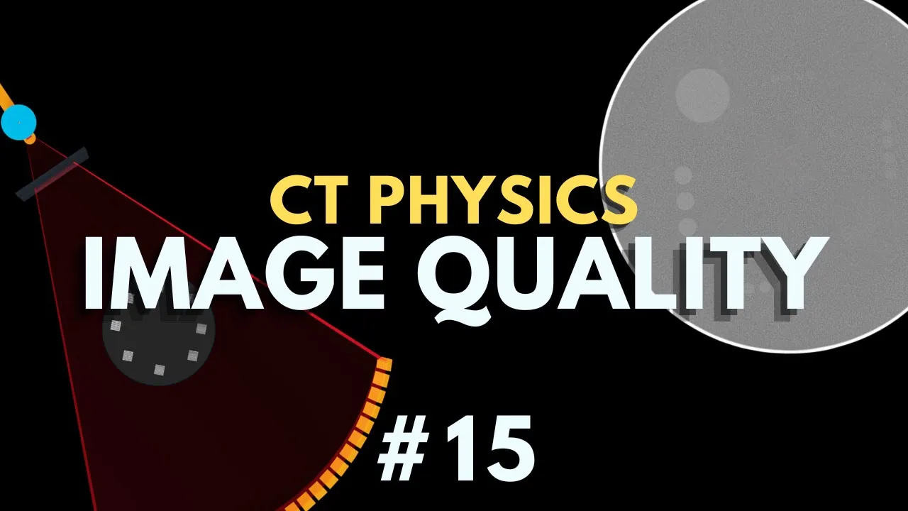





Filtered BackProjection (FBP) is the fundamental algorithm for image reconstruction in modern CT scanners, consisting of two main steps: first filtering the projection data along the detector rows to sharpen edges and reduce blurring, and then performing backprojection where the filtered data is painted back into the image along the original measurement directions; this mathematical method enables accurate conversion from the measured projection data (sinogram) to the final cross-sectional CT image by combining information from multiple views acquired at different angles.
Filtered Backprojection in CT: A Guide for Technologists
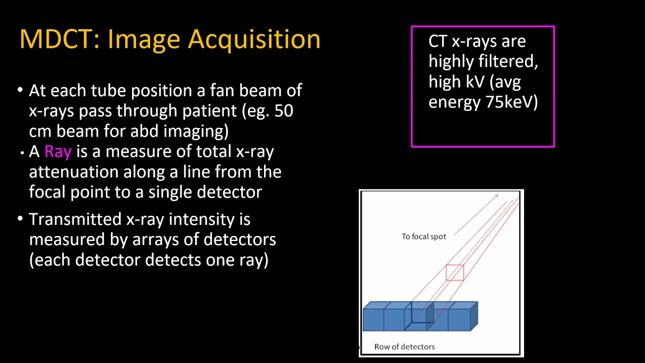
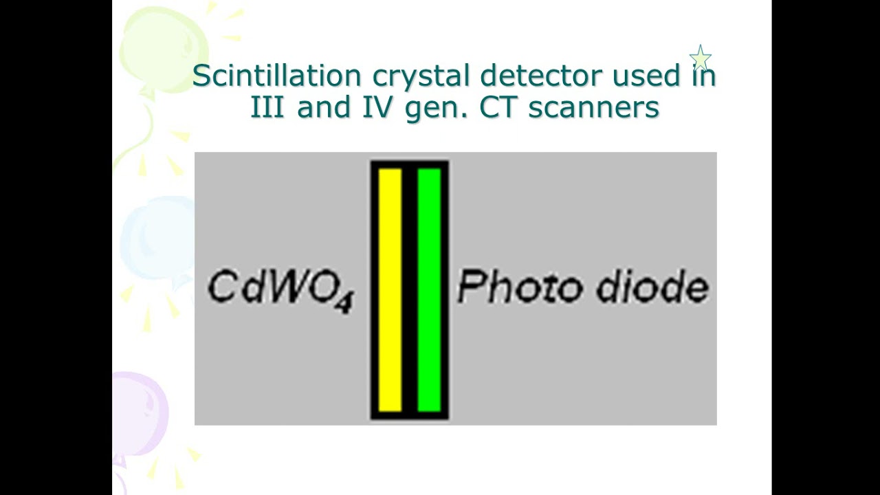
Added:Basic physics of Computed Tomography (CT), including X-ray attenuation and how detector arrays collect projection data.
The geometric concept of a 'projection' and how multi-angle X-ray views are captured during a gantry rotation.
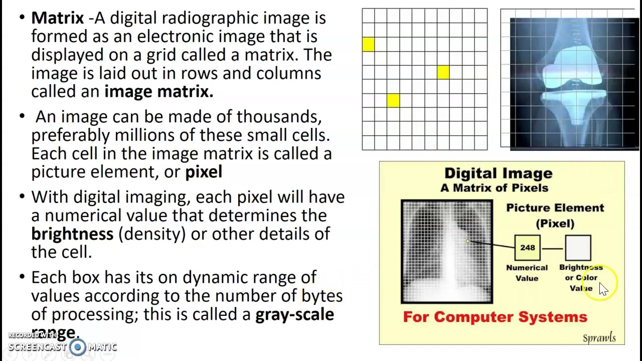
Fundamental digital image concepts, such as pixel grids, matrix sizes, and spatial resolution.
Introductory mathematics of signal processing, specifically the concept of frequency domains and the Fourier Transform.
Iterative Reconstruction (IR) techniques, which are modern, computationally intensive alternatives to FBP that significantly reduce radiation dose.
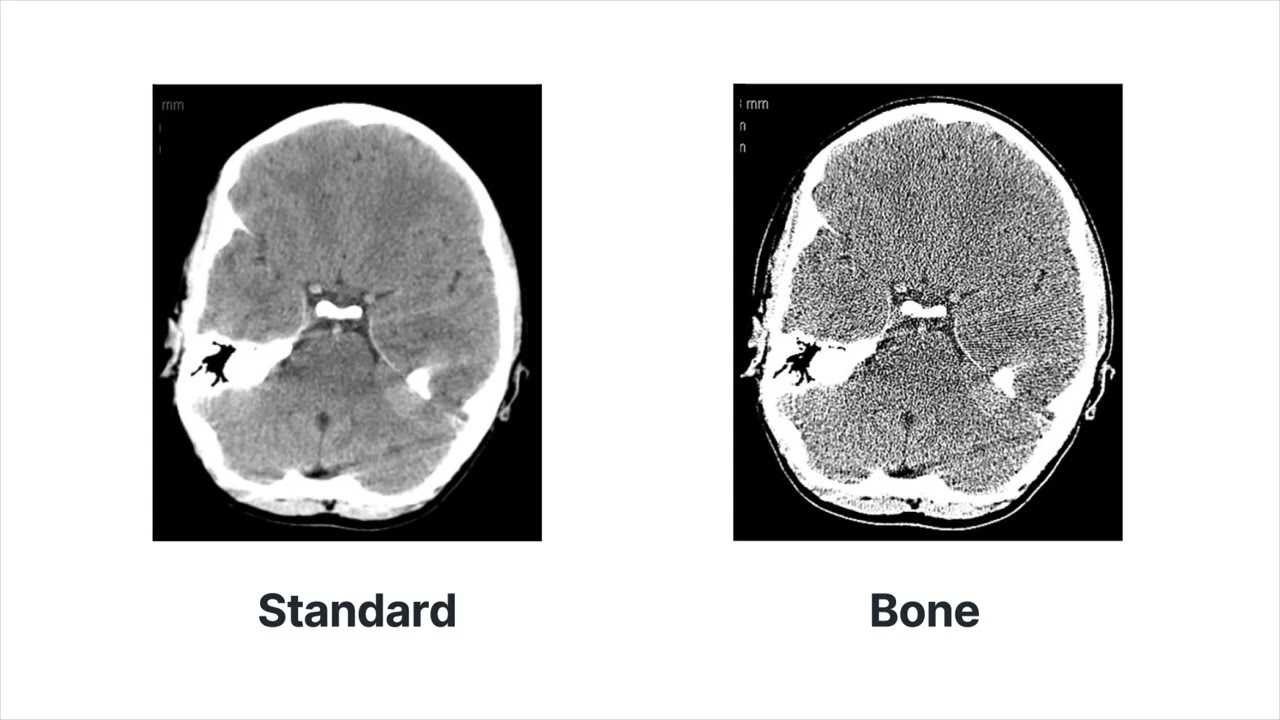
The clinical application of reconstruction kernels (e.g., bone vs. soft-tissue filters) and their trade-offs between image noise and spatial resolution.
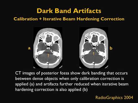
Identification and mitigation of CT image artifacts, such as star artifacts, beam hardening, and aliasing, that stem from reconstruction limitations.
Cone-beam CT (CBCT) reconstruction algorithms, such as the Feldkamp-Davis-Kress (FDK) method, used in dental and radiotherapy imaging.
39.6K views749likes16:01Original Release: 2020-11-27
if you're a radiologic technologist or a student in training working on your art exam or a radiographer and i hear you mumbling wtfbp in the hallway i might think that you're actually wondering what's this filter back projection so in filtered back projection we're talking about how you make images in ct and it can also be used for spect and pet and filtered back projection as the name will tell you really is a simple process of filtering and doing a back projection process we're going to go through the details of what is a projection what's a back projection and why do we need to filter the data and then this image on the upper right just above me is going to make a lot more sense after you stick around all the way through the end of the video filtered back projection coming up [Music] so today we're in the driveway here we're going to be introducing some basic concepts in ct imaging namely forward projection and back projection first i want to introduce myself i'm brian from how ideology works this is bryce from how radiology works and we have a scene here and we're going to describe the different elements of the scene so first you can see back here we have our x-ray source and then here is our image matrix we have our three by three image matrix which is made up of individual image pixels so this is just a 2d matrix so they're image pixels and then inside of some of the image pixels we have our attenuation values so some of these have zero attenuation values and some have attenuation values of one or two attenuation units here and those are going to be measured as by soccer cones and then we have our detector here at the end and you can see this pvc pipe here it's separate into three different regions and that's like our ct detector so that's going to be our scene for our projection and our back projection so now we're going to talk about the forward projection so bryce is going to simulate the forward projection so first he's going to move the x-ray tube and we're simulating what we call first generation ct where the x-ray tube would be collimated and we would go one row of this matrix at a time go ahead so in order to do a forward projection we add up the values all the way along the ray that connects the x-ray tube and our x-ray detector so we started off with one value there and then two values down here so as we draw our straight line between our x-ray tube and our x-ray detector we see that we now have three elements measured in the detector so now bryce is going to go to the second row here so in our first generation ct the x-ray tube would move and then we would take the acquisition so simulating the acquisition here is bryce adding up those so in that case we had just two units and all of the pixels added up along here so we'll come back now and then we'll go to the third row here and we can see in that case we had two units that were in one of the pixels and in this case if we do what we call the forward projection along this row here we see that go ahead brace you see that we have two as well so when we're finally done on our detector we started off with that image matrix that you saw before and all we're going to measure on our detector is three two two so that's all we measure on our detector and that's why having just this one measurement isn't enough to know what was all in the matrix so now we're going to show you another view of the forward projection namely what we were calling the parallel beam forward projection our image matrix is slightly different this time as far as the way we have the attenuation values laid out but essentially the same thing where these are image pixels and then these represent attenuation values and then let's do the forward projection bryce as we go through can you go ahead and do the forward projection of our first row here so again this is the detector here and we see that we had zero zero and three so when we add them all up on the detector it ends up with three in the detector let's move that x-ray tube to the second location go ahead and do this sum along the second location right okay there's actually no attenuation values along that ray so that was an easy one so we had zero along that one and then let's go to the third one and we'll add these up and we add those up and we get three along that direction so you can see that we had the attenuation values spread out in that direction we had one one and one and they all added up to three when we did it from that direction and they all added up to three when they all were three in one location here so you can see that's why we need different views from different angles in order to be able to separate out where the attenuation values truly are in our image matrix if we just have one view we know information about where they're distributed along this direction but we don't know information about where they're distributed along this direction so that's really the bread and butter of tomography and why we want to take multiple views so you saw what happened in terms of the forward projection when we did our actual acquisition along here we added up the values and on our detector we got three zero and three now we're going to show you essentially what the back projection process is so bryce if you want to start down here we'll start down here just like we start on a forward projection and the back projection process is actually just spreading the values along this way evenly so we end up with one one and one as far as the back projection along this row if we're gonna do the back projection of data from the detector so then we'll do the back projection of this middle detector go ahead don't talk and then we got all three added up so now it's zero zero zero and then we'll go to the third one and that detector if we go ahead we're gonna have one one and one so again like we said we're going to need information from multiple views because if we just had this one view if we just do a back projection we can see that the information is spread equally that way and it's spread equally in this direction as well but that's the concept of back projection where you take the value from the detector and you direct it towards where the source projection source position was along which it was measured originally so in this case we showed you parallel beam back projection but the same concept applies with divergent beam back projection except instead of just straight lines through these cells through these pixels you would have divergent beams where the beams would be still connecting the source and the detector so now that we're done with that introduction on the driveway we're coming to the slides and we're going to talk a little more detail about the introduction to projection reconstruction we're focusing on ct here but we do note that there's also other modalities that also will benefit from projection reconstruction but first off what is reconstruction so reconstruction is the idea of taking data those data are in projections and we're going to take those data and do what we call construct or reconstruct the object so if we start with data that's projections through our body we can think of them like shadowgrams to our body we talked about that process of kind of adding up those line integrals so from the source to the detector we're adding up the values along the line that's what we measure on our detector and that's what we're going to take as input to our reconstruction and we're going to do the reconstruction from there there's multiple ways to do the reconstruction there's filtered back projection there's iterative reconstruction and now there's deep learning reconstruction all of these methods can be used to do the reconstruction we're gonna focus today on filter back projection that's been the standard bearer of image reconstruction especially for computed tomography so again just like we said we're talking about ct but then also we note that spect and pet are two other modalities that also have measurements in the projections so in that case we're talking about measurements of the photon decays in spect or of the positrons which then generate photons in pet in both those cases we're talking about surrounding the body with detectors just like we have the body surrounded in ct except nct we only need one side because the x-rays are all coming in one direction from the x-ray tube so the one modality which isn't in here is mri and also ultrasound those are done a little bit differently in mr it's more of a fourier transform and then in ultrasound we're more like back propagating the data along the direction at which it came this is a little schematic where we talk about projections what are the projections so we went through that on the driveway of what is a projection and we're doing the same thing here again showing parallel beam projections again this is through the little bitmoji of my face and we're doing parallel beam projections and for each view you get one projection and then that's one line on this cyanogram so as we see the sonogram the we're talking about given lines and those lines or rows in the synogram they correspond to one view and then the detector direction is the direction left right in that synogram so we can see that after we take several views that we're going to have basically an object that's tracing out in that cyanogram and the objects like if you're at one point in the image it's going to trace out a sinusoidal shape on the cyanogram that's why it's called the cyanogram because the objects in the image are tracing out these sinusoidal patterns luckily we know the direction in which they're tracing so back projection again we talked about back projection in the driveway as well and we talked about the fact that back projection is basically taking the data and spreading it back out evenly so the one issue that we have with back projection is that because it's just spreading that data out evenly what happens is that as we go through and we do back projection for all the view angles if we do that back projection we will end up with an image which looks a lot like the image we're expecting except it looks blurred so that's the key concept that comes out the back projection really helps us to transform from that detector plane back to the image domain but we do need one more step so if you look at that image on the left you can see that the image on the left is a blurred version of the image on the right again the image on the left is going through back projection and the image on the right is what we expect to be for the actual image so we need some sharpening filter so you could think of doing that back projection process and then doing a sharpening filter in the image space and that technically would work especially if you have a large enough detector to make sure you cover the whole object all the time that technically would work except it's just more convenient to do that sharpening in the detector space and again that sharpening we're going to talk about the next slide how we actually do that sharpening but you can have a correspondingly mathematically equal sharpening in the detector space or in the image space and that sharpening filter it's going to go along the rows in the synogram so the cyanogram on the left is the original cyanogram and then the cyanogram on the right is the filtered cyanogram so we can see that the edges are much sharper on that one on the right and that's going to really help us out in order to get then accurate image in the end and what we want to point out here the filter goes again along the row direction so we're filtering along that row direction in the detector domain not in the view domain and we're filtering each row in the detector domain and then that's how we're generating that filtered cyanogram so f in filtered back projection stands for filter again and finally we're going to look at the results of filter back projection we take the filtered views we back project them for all of the view angles in this case we've simulated that parallel beam projections so we have 180 views of data and after we back project 180 views of data you can see that we can faithfully reconstruct that bitmoji picture and we can do so because filtered back projection provides a mathematically accurate method in order to do the reconstruction so it's a significant improvement upon just that back projection image [Music] thanks for hanging around you should also check out our first generation ct video because that has a lot of similarities where we're talking about parallel beam projections
Up Next
16:39
Understanding Viscosity and Shear Stress in Fluid Mechanics
@LetThereBeMath
104.4K views•2017-10-08

30:32
Ultrasonic Transducers: Resonant Frequency Measurement and Horn Design
@imajeenyus42
229.9K views•2017-02-22

54:16
Polymer Environmental Degradation: Mechanisms & Stabilization
@iit
1.8K views•2012-07-10

33:39
How a Student's Question Saved a NYC Skyscraper from Collapse
@veritasium
22.8M views•2025-04-26
Related Study Plans & Knowledge Roadmaps
Structured learning paths in Engineering
engineering
Building Acoustic Levitators: Physics & Arduino
01The Physics of Sound and Standing Waves
02Piezoelectric Transducers and H-Bridge Drivers
03Arduino Programming: Generating 40 kHz Signals
+ 2 more learning modules
14h5 modules
Explore Roadmap
engineering
Building Peltier Cloud Chambers: Particle Tracks
01Cosmic Rays & Cloud Chamber Physics
02Thermoelectric Cooling (TEC) Fundamentals
03Custom Liquid-Cooling Loop Design
+ 2 more learning modules
18h5 modules
Explore Roadmap
engineering
Yagi-Uda Antennas: Modeling, Build & VNA Test
01Introduction to RF and Antenna Fundamentals
02Yagi-Uda Antenna Design Principles
03Antenna Modeling and Simulation in 4NEC2
+ 2 more learning modules
18h5 modules
Explore Roadmap
engineering
ECG Monitor Design: Op-Amps, Filters & Noise
01Electronics & Breadboard Basics
02Op-Amps and Instrumentation Amplifiers
03Bioelectricity and ECG Fundamentals
+ 2 more learning modules
18h5 modules
Explore Roadmap