
























![[와이드경제24] 경제학 짱박사의 와이드경제학 - 6장 독점적경쟁시장과 과점시장 (2)](https://i.ytimg.com/vi/jKTXZurTY9o/maxresdefault.jpg)
In a Stackelberg oligopoly where one firm (the leader) chooses its quantity first and the other firm (the follower) observes and then chooses its quantity, the leader produces more than the follower because it can anticipate the follower's response. Given the demand function P = 100 - 2(Qa + Qb) and marginal cost of $4 for both firms, Firm A (the leader) will produce 24 units, Firm B (the follower) will produce 12 units, and the market price will be $28.
Stackelberg Oligopoly: Quantity Leadership Model Explained
Added:Understanding of the Cournot Duopoly Model, where firms choose quantities simultaneously rather than sequentially.
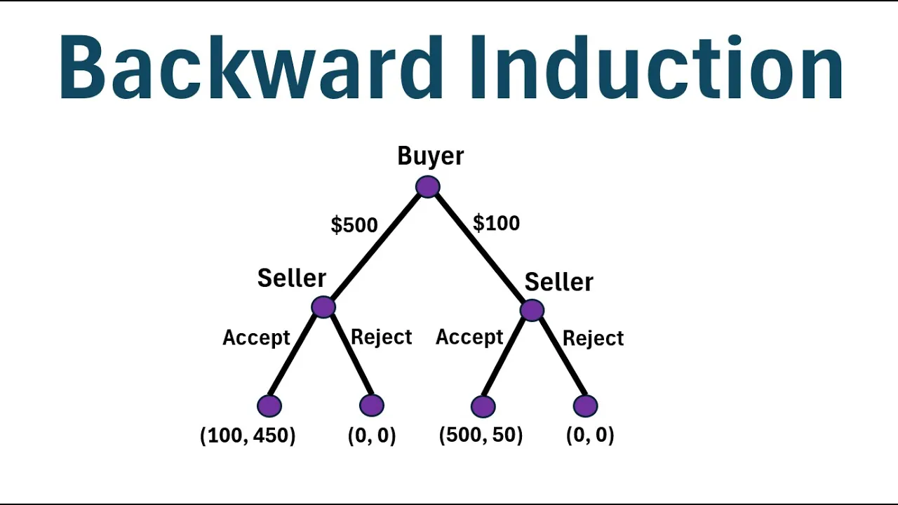
Basic game theory concepts, specifically sequential games, decision trees, and the principle of backward induction.
Microeconomic foundations of profit maximization, including marginal revenue, marginal cost, and demand curves.
Calculus skills, particularly taking partial derivatives to derive a firm's reaction (best-response) function.
Comparison of Stackelberg quantity leadership with Bertrand sequential price leadership models.
In-depth analysis of 'First-Mover Advantage' and identifying economic scenarios where moving second is advantageous.
Extending sequential models to entry deterrence, limit pricing, and capacity preemption strategies.
Exploring repeated games and collusion to see how sequential rivals might cooperate rather than compete.
34.7K views442likes7:42Original Release: 2015-04-11
so I'm going over a quantity leadership problem and in this case there's going to be a marginal cost of production of $4 for both firms and the industry demand is going to be the price of the industry is 100 minus two times the total quantity produced in the industry so we set this up the way we always set up um our maximization problems we maximize by by choosing our choice variable and since this is price leadersh or quantity leadership we're going to use backwards induction and solve firm B's problem first so let's start out with firm B's problem and their choice variable is the quantity that firm B chooses and we're going to maximize as usual price which is the industry price times quantity that we produce that's going to be our total revenue minus the $4 per unit that it cost to create times the quantity we produce and as usual we plug in our demand function so the demand is price equals all this Stu so we're going to plug that in for our price to get um a full form of our profit maximization problem it's going to be 100 minus 2 QA minus 2 QB that's just our demand function which is equal to our price so price times quantity for firm B this is our total revenue now price times quantity minus our total production costs for QB and you can simplify this down using algebra and it's going to give you 96 QB um minus 2 q a QB minus 2 QB 2 and then now we've got our full profit maximization function and we can take our first order conditions to solve for the optimal level of QB and we do that we take the first order conditions of our payoff function with respect to QB as usual and we get 96 minus 2 QA - 4 QB = 0 so when we solve that we find that QB is equal to 24 - 12 QA and this is going to be our best response function and the best response function simply says um whatever firm a does in round one firm B can figure out what should they do by plugging firm A's quantity into this function and it'll tell them what's their optimal decision what's their profit maximizing decision given that so this is our best response function best response function so we've done our first half of our oligopoly problem we know how firm B will respond to from a our next step is to work our way backwards and look at from A's maximization problem and to do that we're going to set up from A's maximization problem and it's actually going to look exactly the same as from B's maximization problem because this is a symmetric problem so from a we'll choose their quantity quantity a by um maximizing the industry price which is the same as it was before it's just our demand function times the quantity that firm a chooses minus the total costs which are $4 per unit times the quantity that firm a chooses to produce so this is now we we've now switched um just by switching the subscripts we we've switched this into firm A's problem and we need to move forth uh let's see we need to move forth and solve it and when we do solve it we are going to solve it by plugging firm B's best response function in we're going to plug this QB up into here and when we do that our profit maximization problem is only going to have qas left in it and they do this really because they they know exactly how their competitor is going to respond so they might as well anticipate that response when they're setting their own price which is why they plug the best response function of firm B into their own maximization problem this is kind of a way for firm a to bully firm B um and as you might imagine in quantity leadership firm a is going to produce way more than firm B will end up producing so let's just make that substitution by plugging this in this can get a little bit boring but um I don't want to skip too many steps since this might be the first time that you've seen this and let's use brackets here around this because we're going to plug it in using parentheses 2 * 24 minus 12 QA so once again this is firm B's best response function and then we have to finish our problem this is price times quantity for firm a minus the total production costs for firm a four dollar per unit times the number of units so now that we have this we can go ahead and solve the whole thing and um when you simplify the the algebra here that whole thing boil actually boils down to something pretty simple 48 QA minus qa^ 2 so very simple this is just solving down the algebra and then you take your first order conditions as usual and take the partial derivative of the payoff function with respect to QA to get 48 - 4 QA set your first order condition equal to Z Z we've got a nice equation with only one unknown and that's going to give us QA when we solve for that the optimal QA is going to be 24 so we know how many units from a will produce so then we need to go back and figure out how many units will from B produce so to do that we need to go find our best response function and I'm going to erase this step up up here and remind us what was our best response function a second ago when we found it and and at that time we found that from B's best response function was that quantity B should be equal to 24 minus 12 of quantity a so if firm a should choose 24 to maximize their profit then firm B is going to choose 24 -2 of 24 24 - 12 and that that's going to be equal to 12 units so that we we know that from B will'll produce 12 12 units and that's not too surprising that the the leader in the industry is going to take up a bigger share of the market than the follower will and now all we need to know is the price in the industry and we find that of course by plugging our QA and QB into our demand function so price equal 100 minus 2 * the total industry quantity which is 24 - 12 and so the price in this industry is actually going to when you solve the algebra be $28 and that was a fully solved uh quantity leadership oligopoly problem
Up Next

160:06
A-Level Economics Paper 1 Revision Tips & Model Answers
@expert.tuition
8.9K views•2023-05-15

5:07
Impact of Yuan in Indo-Russian Trade Amid Sanctions
@WION
261.9K views•2022-07-01
11:06
Adverse Selection vs. Moral Hazard Explained (Economics)
@AshleyHodgson
51.3K views•2020-05-02

113:18
The Age of Easy Money: Fed & Inflation | Full Documentary
@frontline
21.2M views•2023-03-15
Related Study Plans & Knowledge Roadmaps
Structured learning paths in Economics
economics
Sovereign Debt: Defaults, IMF & Restructuring
01Introduction to Sovereign Debt & Government Bonds
02Debt Sustainability & Credit Ratings
03Anatomy and History of Debt Crises
+ 2 more learning modules
12h5 modules
Explore Roadmap
economics
Market Design: Matching Theory & Gale-Shapley
01Introduction to Market Design and Price-Free Markets
02Two-Sided Matching & The Gale-Shapley Algorithm
03School Choice Systems and Mechanism Design
+ 2 more learning modules
10h5 modules
Explore Roadmap
economics
Impossible Trinity: Forex, Capital & Policy
01Introduction to Monetary Policy and Central Banking
02Exchange Rates and International Capital Flows
03The Mundell-Fleming Model
+ 2 more learning modules
8h5 modules
Explore Roadmap
economics
Healthcare Economics: Market Failures & Systems
01Introduction to Healthcare Markets and Market Failure
02Asymmetric Information and Adverse Selection
03Moral Hazard and Insurance Design
+ 2 more learning modules
12h5 modules
Explore Roadmap