Viscoelastic materials exhibit both solid-like and fluid-like properties depending on the timescale of observation; they can be modeled using a combination of springs (representing elasticity) and dashpots (representing viscosity), making them valuable for studying biological tissues like cells that show complex mechanical responses when forces are applied.
Viscoelasticity Explained: Spring-Dashpot Models & Cell Mechanics
Added:Deep Dive
Fundamental concepts of mechanical stress, strain, and shear deformation in materials.

11th Physics | Chapter 6 | Mechanical Properties of Solid | Lecture 2 | Maharashtra Board
46.3K
This comprehensive section covers the foundational concepts of material deformation. Stress is defined as the restoring force per unit area (Force/Area), with SI unit N/m² (Pascal) and dimensional formula [M¹L⁻¹T⁻²]. Strain is the ratio of change in dimension to original dimension, making it dimensionless. The three main types of stress are: (1) Tensile stress - force pulling outward causing elongation; (2) Compressive stress - force pushing inward causing compression; (3) Volumetric stress (hydrostatic pressure) - uniform force over entire surface causing volume change. Correspondingly, the three types of strain are: (1) Longitudinal strain - change in length/original length; (2) Volumetric strain - change in volume/original volume; (3) Shear strain - angular deformation from tangential forces. These concepts form the essential framework for understanding how materials deform under various applied forces.
Click to watch →

Unit -1 || One Shot Video II Introduction to Mechanics of Solid
83.3K
Stress is the internal resisting force per unit area developed when external forces are applied. Normal stress occurs perpendicular to cross-sectional area, classified as tensile (pulling apart) or compressive (pushing together). Shear stress acts parallel to surfaces, causing sliding deformation. Volumetric stress occurs under uniform pressure from all directions. Strain measures deformation as ratio of change to original dimension: longitudinal (ΔL/L), lateral (Δd/d), and volumetric. Poisson's ratio (ν) is the ratio of lateral to longitudinal strain, typically 0.25-0.33 for engineering materials. Shear strain measures angular deformation in radians. These concepts form the foundation for understanding material behavior under loading.
Click to watch →

Strength of Material | Revision in short | SSC JE 2022 | ALOK JHA
19.2K
Stress is a tensor quantity with magnitude, direction, and plane, defined as force per unit area (N/m²). Scalar quantities have only magnitude, while vector quantities have magnitude and direction. Normal stress occurs when perpendicular load is applied, calculated as Normal Force / Cross-sectional Area. Shear stress occurs when parallel load is applied, causing angular deformation. Stress is an internal resistance developed within a body, while pressure is an external force. Pressure can be measured using devices like barometers, but stress cannot be directly measured. Longitudinal axis is where load is applied, while lateral axis is perpendicular to it. Stress occurs only when a body is constrained; if free to expand, strain exists but stress is zero. Strain is the deformation or change in shape/size due to applied stress. Normal strain occurs when perpendicular load is applied, causing change in dimensions (length, width, height). Formula: ε = ΔL/L₀. Shear strain occurs when parallel load is applied, causing angular deformation (change in angle from 90°). Only normal strain causes size change; shear strain causes shape/orientation change. Materials are classified based on elongation: brittle materials (<5% elongation) break suddenly, ductile materials (5-15% elongation) deform significantly before breaking, and very ductile materials (>15% elongation) have exceptional ductility. Brittle materials fail at 90° under tension and 45° under compression, while ductile materials fail at 45° under tension and 90° under compression.
Click to watch →
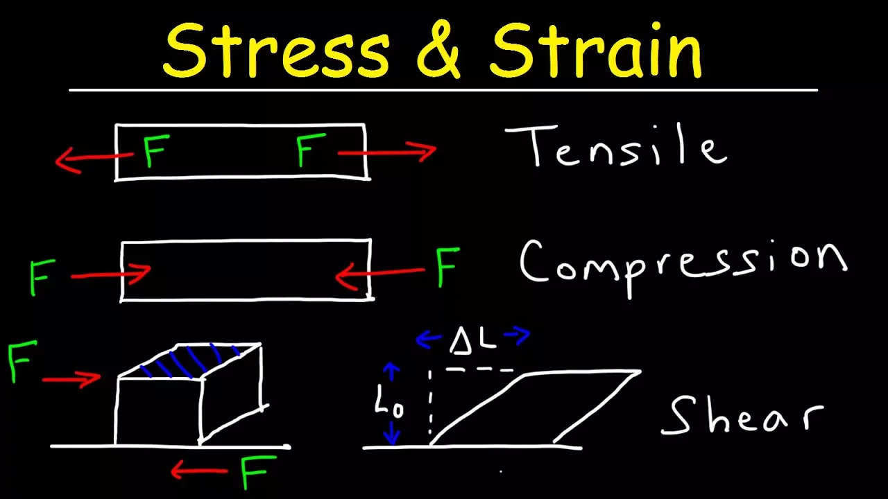
Tensile Stress & Strain, Compressive Stress & Shear Stress - Basic Introduction
837.7K
Stress is defined as force per unit area (F/A), while strain measures the fractional change in length (ΔL/L₀); tensile stress causes elongation with positive strain, compressive stress causes shortening with negative strain, and shear stress causes angular deformation; Young's modulus (E) relates tensile/compressive stress to strain through ΔL = (F × L₀)/(A × E), and shear modulus (G) relates shear stress to shear strain (Δx/h) through similar equations; materials have distinct ultimate strengths—for example, concrete has a maximum tensile strength of 2×10⁶ N/m² and compressive strength of 20×10⁶ N/m², making it much stronger under compression than tension.
Click to watch →

فيزياء الرابع العلمي | الفصل الثاني | المحاضرة 4 | الاجهاد والمطاوعة
1.1K
Stress (الجهاد) is force per unit area, causing deformation (التشوه) in materials. Two stress types exist: longitudinal stress (compression/tension causing length change) and shear stress (tangential forces causing shape change). Strain (المطاوعة) measures deformation and has three types: longitudinal strain (ΔL/L₀), volumetric strain (ΔV/V₀), and shear strain (measured by deformation angle). Strain is dimensionless. The strain type corresponds to the stress type applied.
Click to watch →
Deep Dive
Hooke's Law and the behavior of purely elastic solids (the spring model).

IGCSE Physics Revision: Unit 1 General Physics & Mechanics | for Cambridge IGCSE 2023 Syllabus
256.6K
Hooke's Law states extension is proportional to force (F = kx) within the elastic limit—the maximum force a spring can withstand and still return to original shape. The spring constant (k = F/x) represents stiffness. Students learn to calculate spring constants from force-extension graphs and understand that exceeding the elastic limit causes permanent deformation. This principle explains why springs behave predictably under moderate loads but fail catastrophically under excessive stress.
Click to watch →

فيزياء الرابع العلمي | منهج 2025 | الفصل الثاني | المحاضرة (1) 4K | المقدمة والتشوه وقانون هوك
591.4K
Elasticity is the property of a material to return to its original shape after the deforming force is removed. Springs demonstrate elasticity by stretching when weights are attached and returning to their original length when weights are removed. This behavior arises from attractive forces between molecules that try to restore the material to its original configuration. Robert Hooke discovered the relationship between applied force and resulting deformation, leading to Hooke's Law.
Click to watch →

Hooke's Law JAMB and WAEC Physics and the Elastic Properties of Solids #excellenceacademy
46.8K
Hooke's Law states that the extension produced in an elastic material is directly proportional to the force applied, provided the elastic limit is not exceeded, which can be mathematically expressed as F = ke, where F is the force, e is the extension, and k is the spring constant (measured in Newtons per meter).
Click to watch →

فيزياء الرابع علمي | الفصل الثاني الخصائص الميكانيكية للمادة | محاضرة - 1
513.4K
Elasticity is the property of a material to resist deformation and return to its original shape after the external force is removed. This occurs because the material's molecules try to return to their natural positions. Hooke's Law states that the extension of a spring is directly proportional to the applied force within the elastic limit. This relationship is expressed as F = kΔL, where F is the force, k is the spring constant, and ΔL is the extension. The spring constant represents the stiffness of the spring.
Click to watch →

Hooke's Law explained | झुन्नीलाल की चक्की का Spring वाला तराजू
187.8K
Hooke's Law states that the restoring force exerted by a spring is directly proportional to its displacement from equilibrium (F = -kx), where the spring constant k determines how much the spring stretches or compresses under a given force; when a spring is cut in half, its spring constant doubles because the number of coils is halved, making it stiffer and causing it to show less deformation for the same applied force.
Click to watch →
Deep Dive
Newtonian viscosity and the behavior of purely viscous fluids under shear stress (the dashpot model).
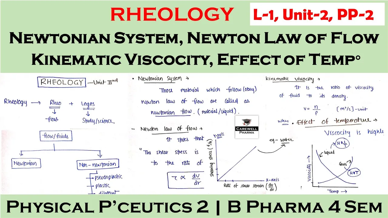
Rheology - newtonian system, law of motion, kinematic viscocity, effect of temp || L-1 U-2 || PP-2
355K
Newton's Law of Viscosity states that for Newtonian fluids, shear stress is directly proportional to the rate of shear strain. Mathematically, τ = μ × (du/dy), where τ is shear stress, μ is viscosity, and du/dy is the rate of shear strain. Shear stress is the force applied per unit area on a fluid surface. Shear strain is the change in angle between adjacent fluid layers when force is applied. When force is applied to a fluid layer, it causes the layer to slide relative to adjacent layers, creating shear strain. This linear relationship defines Newtonian fluids, which include water and most common liquids.
Click to watch →

Compressibility | Fluid and Its Properties - 6 | Fluid Mechanics | #NEGIsir #AIR1 #NEGI10
17K
Newtonian fluid follows the model τ = μ(du/dy), where μ is the dynamic viscosity (constant). For Newtonian fluids, n = 1 in the power-law model. The key characteristic is that apparent viscosity remains constant regardless of the deformation rate. The model passes through the origin when plotted on a shear stress vs. shear rate graph.
Click to watch →

Linear Viscoelastic Materials & Models
34.1K
The linear viscous dashpot model represents viscous behavior using a piston-cylinder arrangement filled with viscous fluid. The constitutive relationship is: ε̇ = σ/η (where η is the viscosity coefficient). Integrating this gives ε = (σ₀/η)t + C, showing linear strain increase with time under constant stress. Unlike springs, dashpots show no instantaneous deformation—strain builds gradually as molecules rearrange. Upon stress removal, the dashpot shows no recovery, leaving permanent strain. This model captures time-dependent viscous flow behavior.
Click to watch →

TOP 55 Most Expected PYQs - Physics | BITSAT 2025 | Score Boost Guaranteed!💯 | Abdul Sir
36K
The shear stress in a viscous fluid is given by τ = η(dv/dy), where η is the coefficient of viscosity and dv/dy is the velocity gradient perpendicular to the flow direction. For a fluid with velocity profile v = k(2y²/a² - y/a), the velocity gradient is dv/dy = k(4y/a² - 1/a). The shear stress is then τ = ηk(4y/a² - 1/a).
Click to watch →
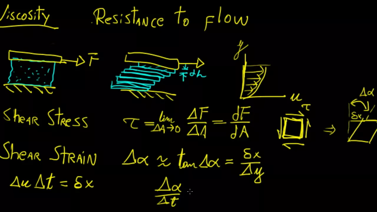
Viscosity and Shear Stress 1 | Fluid Mechanics | LetThereBeMath |
104.4K
Viscosity is the resistance of a fluid to flow, characterized by how fluid molecules adhere to surfaces and move in infinitesimal layers with varying velocities; shear stress in fluids equals dynamic viscosity multiplied by the velocity gradient (τ = μ × du/dy), forming the basis of Newton's law of viscosity for Newtonian fluids, while rotational viscometers measure viscosity by applying torque between concentric cylinders.
Click to watch →
Deep Dive
Basic introductory calculus, specifically ordinary differential equations, to understand time-dependent rates of deformation.

الفصل الثالث / التفاضل / معدلات الزمنية /محاضرة 8 / النوع الأول مساحات والحجوم
131.1K
Time-related rates (المعدلات المرتبطة بالزمن) studies how dimensions change with time while some remain constant. The four-step method: Step 1: Assign variables to changing quantities (فرض المتغيرات باسماء معينة). Step 2: Write the geometric formula relating variables (ايجاد علاقة تربط بين المتغيرات). Step 3: Differentiate with respect to time (اشتقاق العلاقة بالنسبة للزمن تي). Step 4: Substitute known values to find unknowns (التعويض عن المعلوم لايجاد المجهول). Constants should not be assigned variables. Differentiating with respect to time requires writing 'dy/dt' or 'dx/dt' for each variable. For products like x × y = 96, use the product rule: x(dy/dt) + y(dx/dt) = 0. Relationships are divided into primary (the equation being differentiated) and secondary (used to reduce unknowns). Not all problems need a secondary relationship - only when differentiation results in more unknowns than equations.
Click to watch →

الفصل الثالث / التفاضل / محاضرة (32)/ المعدلات الزمنية/تصوير منهج 2024
9.6K
Time-related rates (المعدلات المرتبطة بالزمن) are the first chapter in the calculus textbook, divided into three sections: time-related rates, theorems (Rolle's, Mean Value), and limits. The instructor emphasizes this topic is easier than students think. The five-step method for solving these problems: (1) Assign symbols to dimensions, (2) Find the relevant formula, (3) Identify constants and variables, (4) Differentiate with respect to time, (5) Substitute known values. This systematic approach makes complex problems manageable.
Click to watch →

رياضيات سادس علمي/فصل ثالث/التفاضل/محاضرة 4 / المعدلات الزمنية/شرح تفصيلي/اسئلة النوع الاول/جزء اول
1.1K
This section introduces the fundamental concepts of time derivatives. There are two types of derivatives: ordinary derivative (with respect to variable x) and time derivative (with respect to time t). Time derivatives are used when dealing with rates of change over time. Speed is defined as distance divided by time, making it a time derivative of distance. The rules for time derivatives mirror ordinary derivative rules: derivative of x² is 2x(dx/dt), derivative of y² is 2y(dy/dt), derivative of sin(y) is cos(y)(dy/dt), derivative of e^z is e^z(dz/dt), and derivative of a constant is zero. A time rate of change is a quantity with time in its denominator, such as dV/dt (volume), dA/dt (area), dx/dt (x-coordinate), dy/dt (y-coordinate), ds/dt (distance), and dh/dt (height).
Click to watch →

Cálculo Numérico: Aplicações de EDO numérica - DEFLEXÃO DE VIGA -Seminário
363
Ordinary Differential Equations (ODEs) are equations containing derivatives with one independent variable. They are classified by order (highest derivative: first-order has d/dx, second-order has d²/dx²) and type (ODEs vs partial differential equations with multiple independent variables). The symbol 'd' above variables indicates derivatives. First-order equations produce one integration constant, while second-order equations produce two constants. This classification is essential for solving engineering problems like beam deflection.
Click to watch →

تفاضل - المعدلات الزمنية المرتبطة ( الجزء الاول ) - الصف الثالث الثانوي -م/ محمد كرم عبدالله
3.5K
Time-dependent rates (المعدلات الزمنية) are quantities that change with respect to time, such as the rate of change of length, area, or volume. To solve problems involving time-dependent rates, follow these five steps: (1) Make assumptions by assigning variables to changing quantities, (2) Form the equation relating the variables, (3) Differentiate the equation with respect to time, (4) Stop at the specific moment requested in the problem, and (5) Calculate the final result. The sign of the rate indicates whether the quantity is increasing (positive) or decreasing (negative), while a zero rate indicates the quantity is constant.
Click to watch →
Prerequisite Knowledge
- Concept 01Fundamental concepts of mechanical stress, strain, and shear deformation in materials.
- Concept 02Hooke's Law and the behavior of purely elastic solids (the spring model).
- Concept 03Newtonian viscosity and the behavior of purely viscous fluids under shear stress (the dashpot model).
- Concept 04Basic introductory calculus, specifically ordinary differential equations, to understand time-dependent rates of deformation.
Subsequent Learning
- Step 01Advanced constitutive models of viscoelasticity, such as the Standard Linear Solid (SLS) and Burgers models.
- Step 02Dynamic Mechanical Analysis (DMA) techniques used to measure storage modulus, loss modulus, and viscoelastic damping.
- Step 03The role of cellular viscoelasticity in mechanotransduction, cell motility, and tissue engineering.
- Step 04Polymer rheology and the molecular mechanisms behind polymer relaxation, glass transition temperature, and shear-thinning behavior.
Solid Elasticity
Fluid Flow
Cell Testing
Solid Elasticity
0:01Playing Section
- 1
Solids maintain shape via elasticity, modeled with springs.
- 2
Hooke's Law links force, stiffness, and length change.
- 3
Springs deform temporarily but recover when loads are removed.
Power-Law Rheology and Soft Glassy Rheology in Cell Mechanics
While classic spring-dashpot models (like Maxwell or Kelvin-Voigt) assume cells have a few discrete relaxation timescales, experimental evidence suggests that cell rheology is better described by Power-Law Rheology and Soft Glassy Rheology (SGR). These frameworks argue that the cell cytoplasm behaves like a complex, crowded 'soft glassy material' (similar to foams or pastes) close to a glass transition. Consequently, cells do not exhibit distinct relaxation times; instead, their mechanical response scales continuously as a power law over a wide range of frequencies. This alternative view critiques the simplified linear viscoelastic approach, proposing that fractional calculus or glassy dynamics are necessary to accurately model how living cells deform, remodel, and respond to mechanical forces.
Deep Dive
Advanced constitutive models of viscoelasticity, such as the Standard Linear Solid (SLS) and Burgers models.
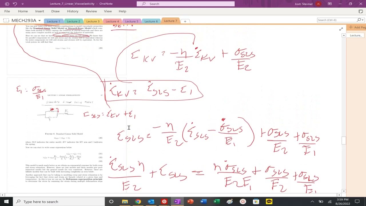
MECH293A: Lecture 7: Standard Linear Solid Constitutive Equation
3.4K
The Standard Linear Solid (SLS) model combines a spring in series with a Kelvin-Voigt model, where stresses are equal across all components and strains sum; its constitutive equation is ε = (σ/E₁) + (σ/E₂) + (η/E₂)(dε/dt), which can be rearranged to ε̇ + (E₂/η)ε = (E₂/E₁)(σ/E₁) + (σ/E₂), enabling analysis of creep and stress relaxation responses by approximating the dashpot as a solid at short times or as disconnected at long times.
Click to watch →
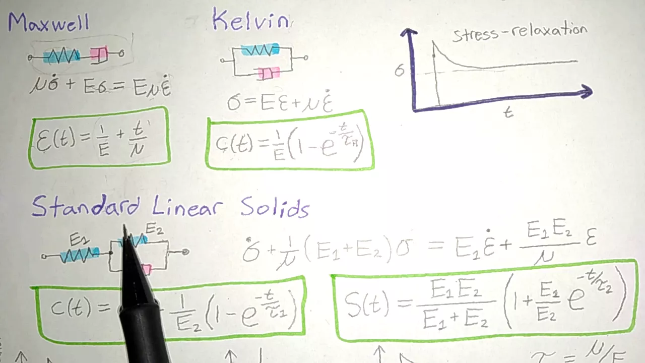
Viscoelastic (Overview and Concept) | Biomechanics
11.6K
Three primary mathematical models describe viscoelastic behavior. The Maxwell model combines elastic spring and viscous dashpot in series, with the relationship: stress rate + (modulus/viscosity) × stress = modulus × strain rate. The Kelvin-Voigt model connects spring and dashpot in parallel, showing strain depends on both stress and strain rate. The Standard Linear Solid model combines both arrangements and best represents biological materials. These models predict different behaviors: Maxwell shows smooth stress relaxation, Kelvin-Voigt shows initial stress spikes, and SLS provides the most accurate representation for real viscoelastic materials.
Click to watch →
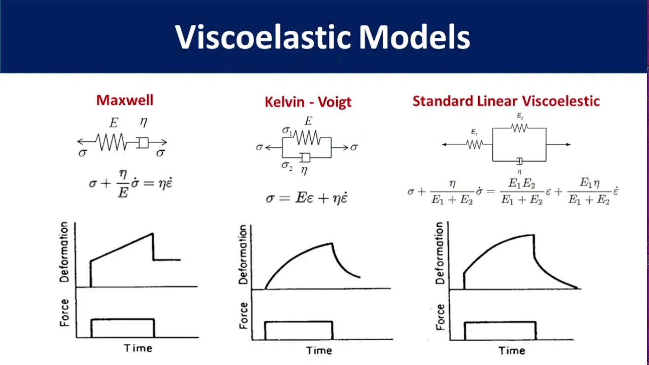
Polymer Viscoelasticity
104K
Three fundamental models explain viscoelastic behavior: (1) Maxwell model (spring-dashpot in series) predicts recovery but fails for creep; (2) Kelvin-Voigt model (parallel connection) accurately models creep but poorly predicts relaxation; (3) Standard Linear Viscoelastic (SLV) model combines both approaches to accurately describe both creep and stress relaxation. These models enable calculation of material constants for predicting polymer behavior under various conditions, essential for engineering applications.
Click to watch →

SafeInCave: Constitutive Modeling of Salt Mechanics
432
Classical models progressively capture more deformation mechanisms: (1) Maxwell model (spring-series-dashpot) captures instantaneous elastic deformation and steady-state creep but misses transient creep; (2) Standard linear solid (spring-series-Kelvin-Voigt) improves transient response but recovers too much upon unloading; (3) Burgers model (spring-series-Kelvin-Voigt-series-dashpot) captures transient, steady-state, and partial recovery but still fails to capture all aspects of salt rock behavior. Each model reveals limitations in capturing the full spectrum of creep phenomena observed in laboratory experiments.
Click to watch →

Seminario viscoelasticidad
105
This section presents fundamental viscoelastic models. The Maxwell model (spring and dashpot in series) predicts indefinite flow under constant stress but no elastic recovery. The Kelvin-Voigt model (spring and dashpot in parallel) predicts steady-state deformation under constant stress but cannot describe creep. The Burgers model combines both, capturing both creep and stress relaxation. Models can use concentrated parameters (constant throughout) or distributed parameters (varying with position). The Deborah number determines which model applies: De >> 1 favors elastic models, De << 1 favors viscous models.
Click to watch →
Deep Dive
Dynamic Mechanical Analysis (DMA) techniques used to measure storage modulus, loss modulus, and viscoelastic damping.
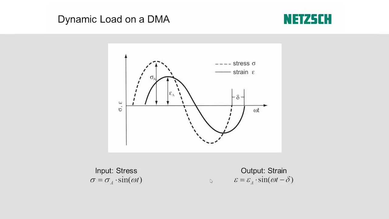
Dynamic Mechanic Analysis (DMA) of Polymers for Beginners
27K
Dynamic Mechanical Analysis (DMA) is a technique that measures the viscoelastic properties of materials under sinusoidal stress as a function of temperature, time, and/or frequency, providing three key parameters: storage modulus (E') which measures elasticity/stiffness and stored energy, loss modulus (E'') which measures plasticity/viscosity and dissipated energy, and loss factor (tan Delta) which characterizes damping/internal friction; this technique is particularly valuable for identifying the glass transition temperature of polymers, monitoring the curing state of thermosets, and evaluating how fillers affect mechanical performance, as demonstrated through case studies on thermoplastic polyurethane, epoxy resins, and carbon nanotube-filled rubber systems.
Click to watch →

What is Dynamic Mechanical Analysis (DMA) or Dynamic Mechanical Testing (DMT)? Principles and Method
7.6K
Dynamic Mechanical Analysis (DMA) is an experimental technique that characterizes viscoelastic materials by applying oscillating stress or strain and measuring the corresponding strain or stress response, enabling determination of key properties such as storage modulus, loss modulus, phase lag (tan delta), and glass transition temperature across a wide range of frequencies (10^-2 to 10^4 Hz) and temperatures (-196°C to 250°C); the method employs two primary approaches—free oscillation (torsion pendulum) which measures amplitude decay through logarithmic decrement to calculate damping properties, and forced oscillation which applies sinusoidal stress/strain and measures phase lag between input and response signals—to study polymer behavior including molecular weight changes, curing progress, and viscoelastic transitions.
Click to watch →
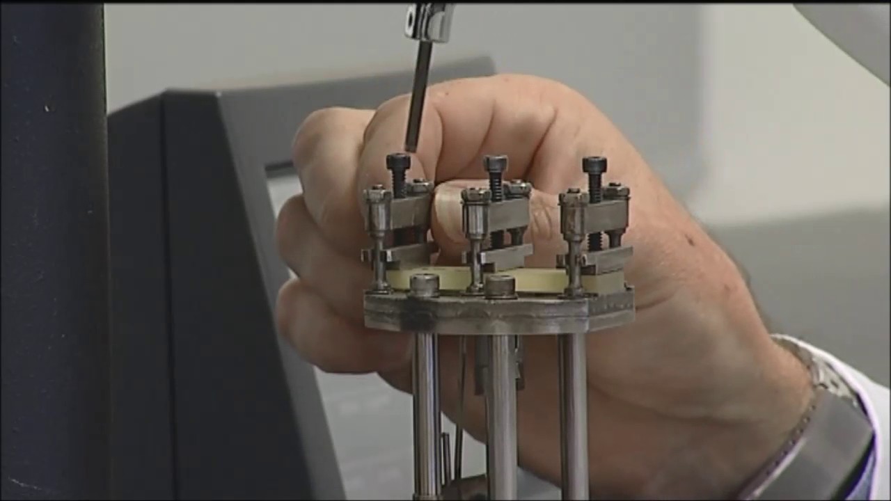
Dynamic Mechanical Analyser DMA
22.8K
A Dynamic Mechanical Analyzer (DMA) measures the viscoelastic properties of polymeric materials by applying oscillatory stress at various frequencies and temperatures, calculating storage modulus (elastic behavior), loss modulus (viscous behavior), and tan Delta (damping ratio); the peak of the tan Delta curve indicates the glass transition temperature, while crosslink density can be derived from these measurements.
Click to watch →

Fundamentals of Damping — Lesson 2
18.4K
Advanced damping characterization addresses complex material behaviors: (1) Viscoelastic damping in elastomeric/rubber materials exhibits frequency-dependent behavior requiring multiple values rather than single constants. Dynamic Mechanical Analysis (DMA) tests provide storage and loss moduli varying with frequency, from which loss factor tan(δ) = loss modulus/storage modulus is computed. Temperature significantly affects damping in non-metallic materials—cold rubber isolators dampen differently than warm ones, similar to cold tires absorbing vibration less effectively. (2) Rayleigh damping provides mathematically convenient linear damping proportional to mass and stiffness matrices: C = αM + βK. Alpha and beta are specified values, not material properties, derived from testing or best practices. Damping ratio varies with frequency due to mass and stiffness contributions, rarely matching requirements across large frequency ranges.
Click to watch →

Dynamic mechanical Analysis|introduction basic principles instrumentation and applications
4.9K
Dynamic Mechanical Analysis (DMA) is a thermal analytical technique that assesses the elastic and viscoelastic properties of materials by applying cyclic stresses and measuring the resulting strain, enabling engineers to characterize material behavior across different temperatures and frequencies; the technique produces storage modulus (E') curves showing elastic behavior and loss modulus (E'') curves indicating viscous damping, which are essential for understanding polymer transitions like the glass transition temperature and optimizing material selection in aerospace, automotive, and industrial applications.
Click to watch →
Deep Dive
The role of cellular viscoelasticity in mechanotransduction, cell motility, and tissue engineering.
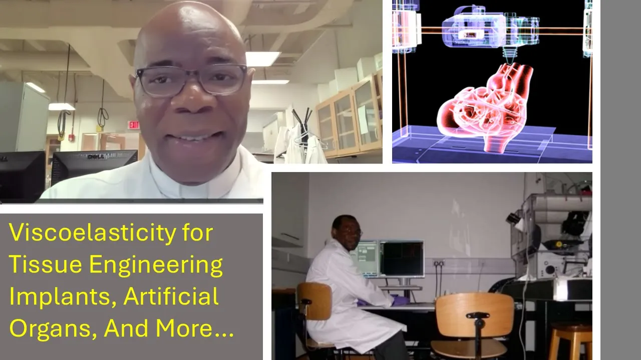
For the Future: Research Recap 2, Viscoelasticity, Tissue Engineering, Regenerative Medicine.
5K
Viscoelastic properties—characterized by both solid-like bouncing back and liquid-like flowing behaviors—are fundamental characteristics of human tissue and individual cells, and research demonstrates that these mechanical properties change during stem cell differentiation into different blood cell lineages, making them fate- and function-dependent markers that can serve as sensitive indicators for monitoring cell differentiation and potential therapeutic targets in regenerative medicine and cancer treatment.
Click to watch →

Cell Migration Seminars #53: Kolade Adebowale & Nicoletta Petridou
1K
When cells interact with viscoelastic substrates, the Young's modulus changes during mechanical loading—initial modulus transitions to long-term modulus. Integrin bonds stretch and build load but eventually fail due to stochastic processes. On fast-relaxing substrates (like pulling a slinky), load builds slowly, allowing time for filopodia formation and maturation. On slow-relaxing substrates (like pulling a car strut), bonds load and fail quickly, disrupting protrusion formation before migration can occur. This explains why cells transition from non-motile on compliant substrates to motile when those substrates have sufficient stress relaxation properties. The key insight is that substrate compliance alone is insufficient—viscoelasticity enables the mechanosensitive cycles necessary for effective cell migration.
Click to watch →

Brandeis Math Bio Seminar - Calina Copos (Northeastern University)
265
Cells can migrate without substrate adhesion through pressure-driven mechanisms, breaking Scallop's theorem by incorporating viscoelastic response in their mechanical description; simulations show that purely elastic boundaries fail to produce net displacement, but viscoelastic boundaries with material turnover enable effective locomotion, which is further enhanced by physical confinement and asymmetric geometries.
Click to watch →

Biointerfaces International 2018 Conference & Seminar, Shoichet/Mooney
269
Cells continuously generate and respond to mechanical forces through actin-myosin interactions, pulling on adjacent cells via cadherins and substrates via integrin-mediated focal adhesions. Mechanical feedback loops involve FAK activating MAP kinase and ROCK pathways, increasing contractility. Mechanical cues directly activate transcription factors altering gene expression. During development, mechanical cues work synergistically with morphogen gradients to regulate pattern formation. Biological tissues are viscoelastic rather than purely elastic, dissipating stresses over time. Physical cross-links enable reversible binding creating viscoelastic behavior, while covalent cross-links create elasticity. Frequency sweep tests distinguish viscoelastic from elastic materials through frequency-dependent modulus. Viscoelastic properties significantly impact cell behavior—rapidly relaxing gels allow cells to spread, migrate, and proliferate, while slowly relaxing gels keep cells rounded. Natural tissues like bone marrow exhibit viscoelastic properties optimal for regeneration. Methylcellulose hydrogels provide injectable, rapidly gelling matrices that maintain uniform cell distribution during injection and provide pro-survival benefits through CD44-mediated mechanisms.
Click to watch →

Scientist Stories: David Mooney, Viscoelasticity From Stem Cell Fate to New Medical Devices
924
This lecture presents research demonstrating that viscoelasticity (the ability of materials to dissipate energy over time) is a critical mechanical cue that regulates cell behavior, including stem cell differentiation, proliferation, and migration, more significantly than stiffness alone; this principle has been applied to develop advanced medical devices such as viscoelastic adhesives that outperform traditional cyanoacrylate adhesives in wet surgical environments and viscoelastic electrodes for neural interfaces that conform to brain tissue geometry.
Click to watch →
Deep Dive
Polymer rheology and the molecular mechanisms behind polymer relaxation, glass transition temperature, and shear-thinning behavior.

#rheology #types of #Flow #plastic#pseudoplastic#dilatant: #classification, #rheogram, #mechanism
6.8K
This section explains the molecular mechanisms behind pseudoplastic (shear-thinning) behavior in polymeric systems. Pseudoplastic systems show entirely nonlinear rheograms beginning at the origin, making single-value viscosity measurements impossible. The mechanism involves polymeric molecules randomly oriented at rest, creating high resistance to flow. Under shear stress, polymer chains align along the flow direction, reducing internal resistance. Simultaneously, solvent molecules associated with polymers become liberated, slightly diluting the solution and further decreasing viscosity. This dual mechanism explains why pseudoplastic materials allow greater shear rates as stress increases, becoming progressively easier to flow under continued shearing. The power-law equation τ = K(γ̇)^n describes this behavior, with n > 1 for shear-thinning systems.
Click to watch →
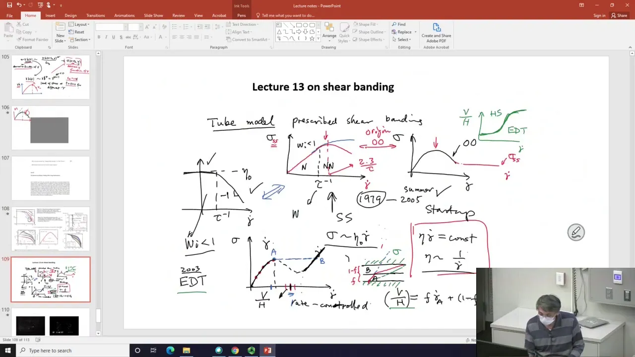
Lecture 19 Essence of Strain Softening: Elastic Yielding 102820
482
This section explains the molecular-level mechanisms behind polymer relaxation phenomena. The tube model assumes chains behave like Rouse chains inside tubes, retracting after stretching to restore equilibrium configurations. Chain retraction causes rapid stress relaxation around characteristic timescales. Over-orientation during initial deformation reduces subsequent stress resistance. Higher shear rates produce greater chain orientation, explaining non-monotonic steady-state behavior. These mechanisms collectively explain overshoot, ultra-strength softening, and rate-dependent effects in polymer systems.
Click to watch →

#23 Glass Transition | Part 2 | Polymers Concepts, Properties, Uses & Sustainability
3K
This comprehensive section covers the fundamental principles of relaxation in polymers, explaining how carbon-carbon backbone bonds rotate to enable macromolecular conformational changes. Materials exhibit multiple relaxation processes operating at different time and length scales, including bond-level, side group, segmental, and overall macromolecular movements, each operating independently. Two fundamental mechanisms govern molecular motion: activated processes requiring energy barrier crossing (following Arrhenius dependence) and cooperative processes exhibiting collective behavior (stretched exponential). Free volume theory explains the glass transition through the concept of free volume—the volume available for molecular motion beyond molecular volume. Below the glass transition temperature (Tg), free volume becomes frozen, preventing segmental mobility. The Williams-Landel-Ferry (WLF) equation quantifies this by relating viscosity at any temperature to viscosity at Tg, introducing a fictitious temperature (T∞, ~50°C below Tg) where viscosity becomes infinite, fundamentally distinguishing glass transition behavior from simpler activated processes.
Click to watch →

回転型レオメーターを用いた粘弾性測定の基礎とポリマー材料への応用 TAインスツルメント 高分子評価レオロジー基礎セミナー
2.9K
Oscillatory rheometry applies small sinusoidal deformations to measure dynamic response through phase angle (δ) between stress and strain. Complex modulus (G*) combines storage modulus (G') and loss modulus (G''). Loss tangent (tan δ = G''/G') indicates damping behavior: low values mean solid-like, high values mean liquid-like. Frequency sweep reveals relaxation processes: low frequencies show long-time behavior (creep, stability), high frequencies show short-time behavior (impact, fracture). Linear viscoelasticity requires staying within the linear regime where response remains sinusoidal. The glass transition temperature (Tg) marks the amorphous-rubbery transition, identified by tan δ peaks or G'/G' crossing points. Polymer characterization uses rheology to relate molecular structure to macroscopic properties. Zero-shear viscosity follows η₀ ∝ M^3.4 for linear polymers. Molecular weight distribution affects plateau modulus (G₀)—broader distributions produce lower plateau moduli. Branching increases entanglement density and raises both η₀ and G₀. Relaxation spectra reveal multiple relaxation processes corresponding to different molecular motions. Crosslink density affects Tg and tan δ, balancing tack with cohesive strength in adhesive formulations.
Click to watch →

Rheology for educated beginners – Rheology 101
151
Shear thinning describes how viscosity decreases under higher shear rates. Long polymer molecules coil at rest but align and extend in flow directions, reducing resistance. This explains why toothpaste flows easily through narrow openings but remains thick when at rest. Single-point measurements miss critical behavior—proper characterization requires testing across multiple shear rates. Practical implications include food handling (honey drips continuously while marmalade stays put) and industrial processing efficiency.
Click to watch →
Solid Elasticity
Fluid Flow
Cell Testing
Solid Elasticity
0:01- 1
Solids maintain shape via elasticity, modeled with springs.
- 2
Hooke's Law links force, stiffness, and length change.
- 3
Springs deform temporarily but recover when loads are removed.
Power-Law Rheology and Soft Glassy Rheology in Cell Mechanics
While classic spring-dashpot models (like Maxwell or Kelvin-Voigt) assume cells have a few discrete relaxation timescales, experimental evidence suggests that cell rheology is better described by Power-Law Rheology and Soft Glassy Rheology (SGR). These frameworks argue that the cell cytoplasm behaves like a complex, crowded 'soft glassy material' (similar to foams or pastes) close to a glass transition. Consequently, cells do not exhibit distinct relaxation times; instead, their mechanical response scales continuously as a power law over a wide range of frequencies. This alternative view critiques the simplified linear viscoelastic approach, proposing that fractional calculus or glassy dynamics are necessary to accurately model how living cells deform, remodel, and respond to mechanical forces.
Fundamental concepts of mechanical stress, strain, and shear deformation in materials.
Hooke's Law and the behavior of purely elastic solids (the spring model).
Newtonian viscosity and the behavior of purely viscous fluids under shear stress (the dashpot model).
Basic introductory calculus, specifically ordinary differential equations, to understand time-dependent rates of deformation.
Advanced constitutive models of viscoelasticity, such as the Standard Linear Solid (SLS) and Burgers models.
Dynamic Mechanical Analysis (DMA) techniques used to measure storage modulus, loss modulus, and viscoelastic damping.
The role of cellular viscoelasticity in mechanotransduction, cell motility, and tissue engineering.
Polymer rheology and the molecular mechanisms behind polymer relaxation, glass transition temperature, and shear-thinning behavior.
167.4K views844likes4:50@bamlab6787Original Release: 2013-09-18
We describe most materials by the properties they exhibit Fluids take the shape of their container Solid materials tend to hold their shape If it's soft, a solid can deform... But will eventually return to its original shape The ball changes shape as it bounces off the table But eventually returns to its original shape This property is known as ELASTICITY We can model the elasticity of solids using a spring The spring stretches a fixed amount when a weight is added This is caused by the gravitational force on the weight Additional weights cause the spring to stretch by the same amount We can calculate the spring's stiffness using Hooke's Law Force = Spring stiffness x Change in Length A spring's stiffness changes very little So the spring returns to its original position after the weights are removed Both liquids and gases can have fluid-like properties Like liquids, gases take the shape of their container They can also be poured out of their container too Unlike solids... Fluids respond to forces by continuously moving We can use a dashpot to model this property Force = Fluid viscosity x (Rate of change of Dashpot Length) When weights are added, the dashpot continues to deform Unlike the spring, after the weights are removed, the dashpot does not return to its original shape Many everyday things we use have both fluid and solid like properties Some of these materials are called VISCOELASTIC Did you know that silly putty is a viscoelastic material?
It acts like a solid if you bounce it quickly... But flows like a liquid over a long period of time These materials are important because they can be used to model the tissues that make up you and me!
We can tell that cells are viscoelastic by pulling on them, using a magnet The response of a bead attached to a solid surface is similar to that of a spring In contrast, the response of a bead attached to a cell is more complex The bead moves towards the magnet when it's turned on, but relaxes when the magnet is turned off Now let's look at a bead attached to the surface of a live cell When the magnet is turned on, the response is similar to that of a dashpot But when the magnet is turned off, the bead returns to its original position (like the spring) Viscoelasticity can be modeled by a spring and dashpot in parallel By adjusting the spring and dashpot properties to match the deformation of a material We can decompose a single response to see how much of a material is a solid or fluid We can model changes in cell stiffness, or identify cells based on their viscoelastic properties
Up Next

8:00
Hemodynamics Explained: Blood Flow, Resistance & Cardiac Output
@10minutephysiology50
610 views•2023-02-17

12:53
21cm Hyperfine Transition in Neutral Hydrogen: Radio Astronomy Basics
@AaronRobertParsons
12.4K views•2011-10-13

32:32
NMR Spin Physics I: Zeeman Effect, Resonance Condition & Larmor Frequency
@nptel-indianinstituteofsci8064
2.3K views•2024-01-17

27:14
Entropy and the Second Law of Thermodynamics Explained
@veritasium
27.5M views•2023-07-01
Related Study Plans & Knowledge Roadmaps
Structured learning paths in Physics
physics
Nuclear Physics (Decay, Fission & Reactors)
01Atomic Structure and the Binding Force
02Radioactive Decay and Half-Life
03Nuclear Fission Mechanics and Chain Reactions
+ 2 more learning modules
12h5 modules
Explore Roadmap
physics
Soft Matter (Polymers, Colloids & Rheology)
01Foundations of Soft Matter & Thermal Forces
02Polymer Physics and Macromolecules
03Colloids, Surfactants, and Self-Assembly
+ 2 more learning modules
38h5 modules
Explore Roadmap
physics
Analytical Mechanics: Lagrangian & Hamiltonian
01Mathematical Foundations: Calculus of Variations
02From Newtonian Mechanics to Constraint Dynamics
03The Principle of Least Action & Lagrangian Mechanics
+ 3 more learning modules
28h6 modules
Explore Roadmap
physics
General Relativity (Spacetime & Cosmology)
01Foundations of Relativity: Special Relativity
02The Geometry of Spacetime: Equivalence Principle & Curvature
03Einstein's Field Equations: The Mathematics of Gravity
+ 2 more learning modules
55h5 modules
Explore Roadmap