







![[임베디드 기초 뿌수기 강좌 2-5] 임베디드에서 무조건 쓰이는 구조체와 포인터](https://i.ytimg.com/vi_webp/IIdVC4Yc1fQ/maxresdefault.webp)







This video demonstrates how to implement an Extended Kalman Filter (EKF) in real-time on an STM32 microcontroller for sensor fusion, covering the complete workflow from low-level firmware setup (including MPU6050 driver, DMA, and USB logging) through axis remapping, sensor calibration, and low-pass filtering, to the EKF algorithm itself which involves initialization, prediction using Euler integration and Jacobian matrices, and update steps with Kalman gain calculation. The implementation uses symbolic computation in Octave to derive matrix operations and shows practical considerations like parameter tuning (Q and R matrices), sample time selection, and trade-offs between filtering effectiveness and system lag.
Extended Kalman Filter Implementation for Sensor Fusion | STM32 C Tutorial
Added:Fundamental understanding of the standard Linear Kalman Filter, including state estimation, covariance matrices, and the predict-update cycle.
Basic multivariate calculus and linear algebra, specifically matrix multiplication, inversion, and calculating Jacobian matrices for linearization.
Physics of Inertial Measurement Units (IMUs), including how accelerometers and gyroscopes function, and their respective noise and drift characteristics.
Proficiency in C programming for embedded systems, including structures, pointers, and basic peripheral communication (I2C/SPI) on STM32 microcontrollers.
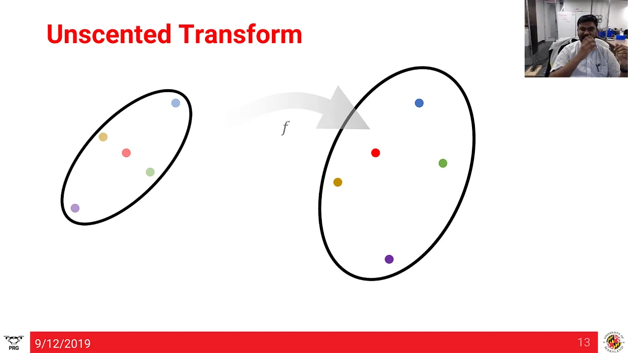
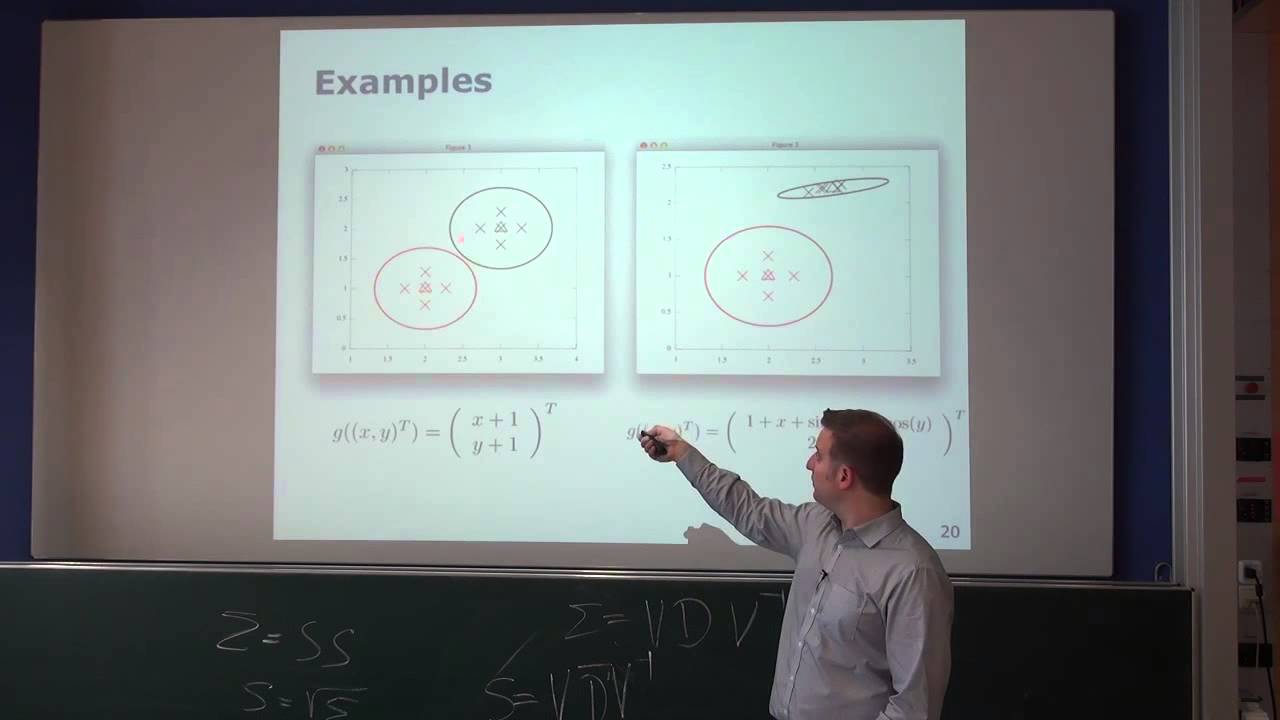
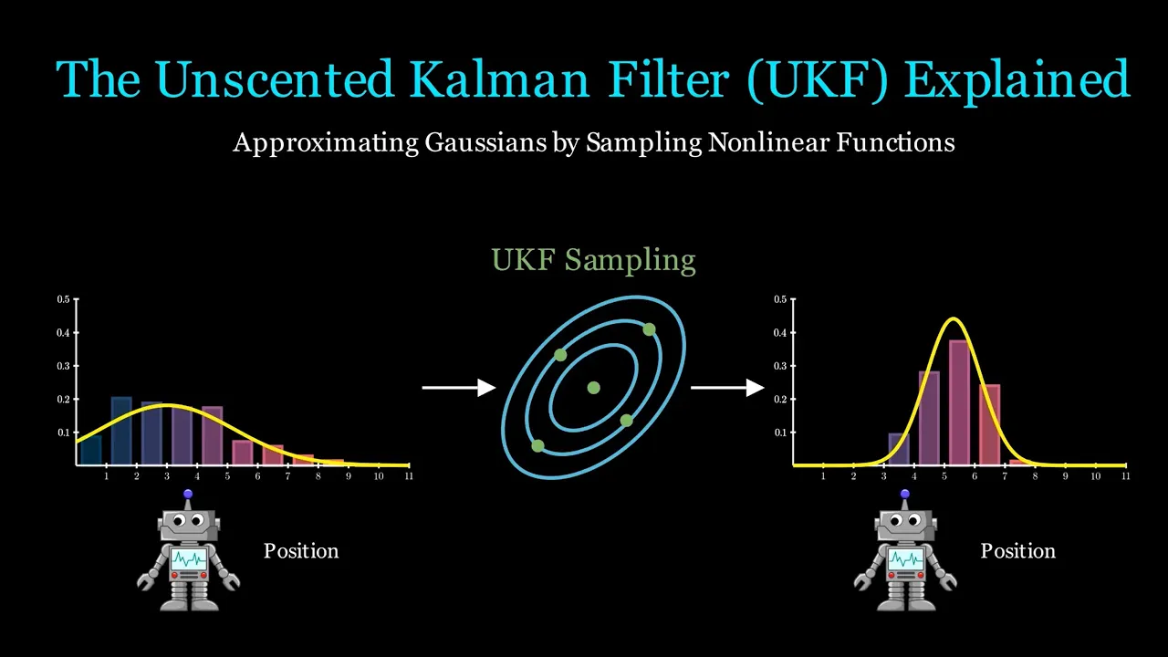
Exploring the Unscented Kalman Filter (UKF) to handle highly non-linear system dynamics without calculating analytical Jacobians.
Integrating a 3-axis magnetometer into the state vector to create a 9-DOF Attitude and Heading Reference System (AHRS) to resolve heading drift.
Studying multi-sensor fusion architectures, such as coupling GPS/GNSS data with the IMU EKF for robust inertial navigation (INS).
Optimizing EKF execution on resource-constrained microcontrollers using hardware floating-point units (FPU) and the ARM CMSIS-DSP library.
72.2K views1.8Klikes28:56Original Release: 2022-08-22
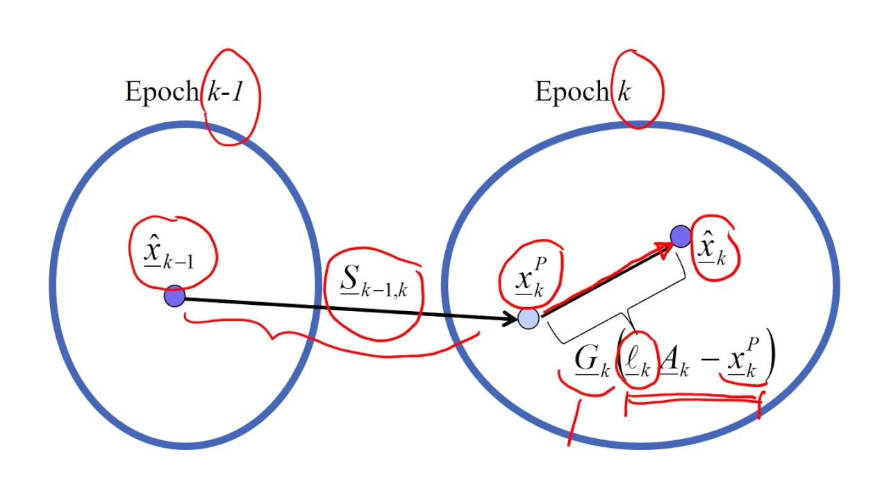
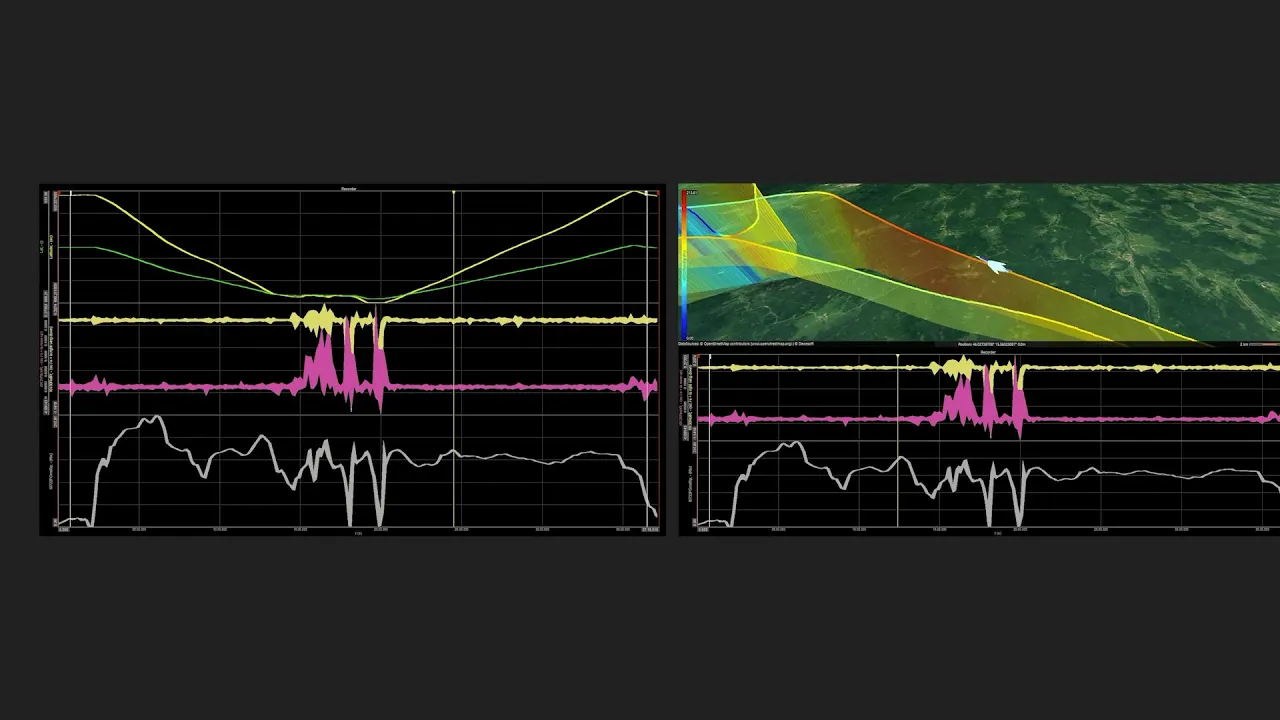
in this video we'll be looking at how to implement an extended kalman filter in real time in software on an embedded system in particular we'll be looking at this little brain plus plus board featuring an stm32f4 microcontroller and programming in c this is the last part of the sensor fusion series of videos so make sure you've checked out the previous three videos to get familiar with the topic thank you very much to altium for sponsoring this video the little brain pcb you saw at the beginning was designed using autumn designer if you'd like to give altium design a try for yourself you can get a free trial if you go to autumn.com forward slash yt forward slash phil's lab if you're interested in the hardware design aspect of this little brain plus plus board i have a video number 38 giving you an overview of the hardware design in autumn designer thank you also to jlc pcb for sponsoring this video i had the little brain plus manufactured and assembled by them if you'd like to get yourself a little brain plus plus board or look at the design files you can go to my github account at github.com forward slash pms67 and then navigate to the little brain plus plus repository you can find all the altium design files assembly and gerber files over there this is the last part of the sensor fusion series and of course there'll be some prerequisites that i'll be basing this video on please watch the previous videos on sensor fusion first of all we have the sensor fusion introduction video on my channel this is number 33 called accelerometers and gyroscopes we had a look at the complementary filter which is one of the most simple types of observers or sensor fusion algorithms and this is video number 34 on my channel which also goes into the real-time implementation using stm32 microcontrollers lastly we looked at the extended kalman filter or ekf theory and a lot of this video will be based on this third video so please make sure to check that out as i won't be going over the theory in this video this video then only covers the actual ekf implementation in real time the last ekf video was number 37 on my channel in this video we first have to look at the low level firmware before we even get to the ekf part this includes the microcontroller setup so selecting the pin out doing the hardware extraction layer via stm32 cube ide then we need to write a driver for the mpu6050 and i'm using i squared c in this example but i squid c really shouldn't be used for any mission critical or critical systems at all other than really simple configuration then we need to read the data via dma once we have these data read and the dma gives us an interrupt flag we need to call an ekf processing function and if you remember from the last video we have both predict and update functions in our kalman filter another option of doing this would be using a real-time operating system and i've just gone the really simple route just for demonstration purposes we also need to ensure accurate timing and fixed sample rates lastly our firmware for demonstration purposes should log data via usb now i do have several videos on all these topics which i'll link to in the description below so make sure to check those out how to do proper mcu setup writing a driver and doing dma and usb logging i'll just gloss over the main functions in this video as you saw the start of this video i'm implementing this firmware on the little brain plus plus board which contains an stm32f411 microcontroller and i've already done the pin out for this so i've been enabled external crystal oscillator i've enabled usb full speed i squared c my imu interrupt and serial wire debug i have some other peripherals for different sensors but we won't need this in this video in middleware i've also enabled the usb device as my communication device class which is a virtual comport if you're interested in looking at this in more detail i have a brief video on scm32 board bring up that's video number 54 which goes exactly over the bring up of the basics of this little brain plus plus board of course i have more involved videos on my channel again i'll leave the link in the description below we can briefly look through the main.c code before we move on to the actual ekf implementation i'll just briefly show you the imu driver as well for completeness sake the imu drivers for the mpu6050 and i've written a really crude driver i didn't even write a dot c file it's all in container.h file i'm just storing various register addresses which i need to enable the inertial measurement unit to power it up and then the registers for reading the data also some various conversion factors because i read essentially raw data from the inertial measurement unit and i want to convert that for example the accelerometer data from raw to meters per second squared so i have this magic factor over here i want my raw gyroscope data to map to radians per second so rps i'm storing all of this data in a struct and then i initialize the sensor to the proper four parameters that's the acceleration range is plus minus 2g and gyroscope ranged plus minus 250 degrees per second now this of course will vary depending on the situation you're in if you're placing this in a very maneuverable drone it's very likely that you'll have ranges far higher than these but since i'm just playing around with this on my desktop default ranges are perfectly fine i am also enabling the internal digital low-pass filters even though we'll be performing some low-pass filtering in software later to have a sample rate of one kilohertz and i'm limiting my accelerometer bandwidth to 94 hertz and gyroscope to 98 hertz again this is situation dependent then i'm setting up the interrupt to make sure every time data is ready my interrupt flag is set and then i can trigger the dma read that's all there is to this initialization function i then have essentially the process or read data functions one is the read dma which essentially just calls the hardware abstraction layer read dma and reads all the accelerometer and gyroscope data then sets that read ready flag i also have a small process data function which simply converts from my raw data to my process data and we'll come back to this because we also have to do an access remapping in main.c there's not much special i'm including my usb drivers my 6050 drivers and then the extended kalman filter source file which we'll go over later my various constants which i'll examine later as well some things to note are sample times in milliseconds so i've already set up my predict and update periods as well as my usb logging period as well i have an interrupt handler as my callback so every time anytime the mpu 6050 has data ready it pulls a pin high this interrupt handler then says okay data is ready let's perform a dma read once we've performed the read essentially i clear the data ready flag and then i process the imu data in int main we just have the usual hal setup we initialize the mpu-6050 we initialize the kalman filter again we'll come back to this later and then we have our main while loop i haven't used an rtos and this is a pretty crude implementation especially timing wise i'm just checking with timers if a certain time has elapsed and then calling functions for example filtering my imu data or my prediction step of the common filter my update set with the cam filter logging and toggling an led you can see in the logging function i'm just using the hardware extraction layer or the virtual comport device class i'm simply sending my roll and pitch values compared to converted from radians to degrees via usb so rather crude very basic setup all i'm setting up is dma streams sensors and then fixed timing intervals to send data and also to process the ekf data and that's all there is to this base firmware as i've hinted at previously we have to do some things before we go into the actual ekf implementation one of these is accessory mapping if you remember back to our previous videos our ekf algorithm including the sensor model we used for example for the gyroscopes and accelerometers assumes a particular orientation of axes and this happens to be shown on the right here we have x as north y is east and z is down however the initial measurement unit we're using in particular the mpu 6050 has its own set of axes and this is taken from the datasheet shown here and you can quite clearly see this mapping is completely different so what we have to do is make sure that the mpu6050 mapping maps to the ekf algorithms model which is assumed otherwise we're going to get completely rubbish data out this is actually fairly straightforward now there's better ways of doing this rather than just doing this in the mpu6050 driver of course because this driver might be used in a completely different project but since i have this pretty much just local to my etf i've just put it in here anytime i set my structs accelerometer values i take my raw data and then remap it for example changing the sign and also saying the x-axis is actually the mpu-6050's y-axis or the ekf y-axis is actually the mpu 6850x axis and so forth i need to do that both for the accelerometer as well as for the gyroscope calibration is a huge topic in its own right and i'm just going to briefly gloss over it with this slide but keep in mind this is one of the most crucial factors for having a successful sensor fusion implementation raw sensor measurements are typically biased or distorted in some way so the sensor measurements need to be calibrated ideally this should be performed every start up or at least periodically this is to remove offsets which are typically known as biases and scaling errors in essence we have a linear mapping we will perform in the most simple case we have our raw sensor data we have to adjust it with a scale and add a constant or bias to it to get our calibrated measurement value which we then feed into our remaining algorithms in essence for gyroscopes the easiest way we can do this is keep the gyroscope to the rest average the readings so add up all the readings divide by the number of readings you have and find c bias or the offset for every axis then later on we can subtract c bias from every measurement to have our calibrated measurements for the accelerometers that's a bit more complicated we need six measurements at least so each axis aligned in either direction positive and negative and this allows us then to find the scale factor and the bias value of course you can imagine keeping these devices at rest will be hard with external influences as well as aligning these axes properly to give us plus minus g in either direction so calibration is a huge topic and typically requires specialized equipment to perform properly another aspect is that we saw in previous videos is that the raw accelerometer and gyroscope readings after they've converted from the very raw values from the mpu6050 to meters per second squared and radians per second these will contain additive high frequency noise and this is pretty much unavoidable so you could get higher quality sensors which will in turn be more expensive you can use a lower bandwidth digital filter for example directly in the ic and we're essentially doing the same thing it always pays off to do some additional measurement processing in terms of low pass filtering and this applies both to the accelerometer as well as a gyroscope we use a low pass filter the measurements before passing these to the ekf from previous videos you will know any reasonable and fast filter is a simple first order iir filter digital filter employing feedback i have an extended video on irr filter design on my channel again i'll leave a link to this in the description below in essence filter we're using before we're passing these measurements to the extended kalman filter is this simple discrete time difference equation at the bottom here our output is y at sample n and our input is x of n so x of n would be our raw accelerometer and raw gyroscope data and of course we need three channels of accelerometer and three channels of gyroscope so we'll have six instances of this filter alpha is our filtering coefficient which goes anywhere from zero to one if we have alpha equals zero we essentially we have no filtering and y of n is x of n so the output is the input of the filter as alpha goes towards one we take more of the previous output of the filter into account rather than accepting the input so as alpha goes to one we perform more and more filtering as is usual with sensor fusion there's no direct way of determining alpha and this is something we have to play around with and also tune in the software implementation in my main while loop i'm checking if the imu data ready flag has been set and the dma transfer is not currently in progress if that's the case i can filter my imu data remember we have to do this for all of the gyroscope data and all the accelerometer data i've defined a low-pass filter gyroscope alpha and accelerometer alpha you typically want to keep these separate gyroscope data contains a lot of high frequency information so you don't want to filter that as heavily as for example the accelerometer data and that's why the gyroscope alpha is 0.01 in this case and the accelerometer alpha is 10 times higher at 0.1 of course you'd have to play with these values all i'm then doing is then implementing the difference equation so the current filtered gyroscope data is the previous gyroscope data times the alpha plus 1 minus the alpha times the current gyroscope data same thing for the accelerometer we're pretty much ready now to look at the ekf algorithm in particular the implementation let's remind ourselves of the algorithm essentially three steps two of them repeating the first is to initialize the ekf so we have a state estimate in our case we're trying to estimate rule and pitch angles so our state estimate is x hat at sample time zero and of course x hat is a vector because it's rolling pitch p q and r are matrices so p is our essentially error covariance of the current state so how uncertain the algorithm thinks our state estimates are q and r are noise and error matrices q for the process and r for the measurements we also need to define a sample time so what time is the between prediction steps and what time is there between update steps predict and update oftentimes can come together but usually they are separate for a prediction step we'll have sensors that update frequently for example the gyroscopes and our update step we might have sensors that update slowly this could be gps units lidars and so on our prediction step will be concerning the gyroscopes and our update step will be concerning the accelerometers the prediction step we have our state transition function f of x and u which is essentially the rate of change of our model of of the state estimate so it's x dot we can perform simple euler integration x dot times t plus the previous date gives us our new state and that's our prediction step again all this was covered in the previous video we then also have to update our error covariance matrix using this formula below here and we'll see exactly how to implement that numerically or how we get an actual expression that we can implement in a programming language in just a second our update step is different we have to compute the kalman gain and this unfortunately involves a matrix inversion luckily for us we will only have to invert a 3x3 matrix but you can imagine how expensive this operation is for largest system dimensions then we apply the correction step which is essentially the common gain depending on our accelerometer measurements and this depends on the common gain as well and then again we have to update our error covariance matrix let's look at the initialized step first to initialize we initialize our state estimate and this will contain the role at time zero and the pitch at time zero and for most cases we'll just set these to be zero i'm having my board lie flat on my table and i'm assuming that's a roll and pitch of zero of course the table could be misaligned the sensors misaligned so on this is our initial state estimate so really easy to set up we could of course use the accelerometer to give us initial state estimate giving a very crude estimate of inclination and roll then we have the error covariance matrix and it's starting to become a bit more complicated p our error covariance matrix gives us an estimate of how uncertain our estimates are initially p should be diagonal and typically small non-zero elements and the order of magnitude might be something 0.1 0.01 that kind of ordered magnitude it's hard to generalize we also have our process noise and measurement noise matrices these are q and r respectively and typically these will be diagonal and in our case we will not change them with time but it's very sensible and often times to make these time varying the elements of q the diagonal elements can be determined by the variance of the process noise so that takes into account our sensors in the model and the elements of r are termed by the covariance of measurement noise including the sensors and model again now this is a very high level description of how to determine q and r and often times in practice and even though you might be able to get them directly from the model and sensor data sheets in practice you will have to do quite a lot of tuning of q and r to make sure your ekf performs appropriately if q and r aren't set properly your state estimates will diverge it'll be an unstable filter and so on so it pays off to spend some time tuning q r lastly of course you also have the sample time predict and update steps will be sensor dependent it depends on when we get our rate updates from the gyroscopes or when we get our accelerometer measurements and these might be different sample times in any case the sample time should be as small as possible especially for the prediction step we get better numerical integration accuracy especially with such a simple oil integration method this of course is limited by the processing power now for the first time let's look at the actual code of the kalman filter implementation this is incredibly crude very simple and simply for demonstration purposes again this shouldn't be used in any sort of critical system this is the header file and we have three functions initialize predict and update as well as this struct the common field of struct takes our state estimates i in radians and theta in regions that's roll and pitch respectively it takes our error covariance matrix which is a 4x4 matrix our process noise matrix q which is a 2x2 matrix and our measurement noise matrix which is the 3x3 matrix r the initialization function then takes the struct one initial value the error covariance and this will place this value along the diagonal and then pointers to q and r matrices in the actual function itself we can see we're initializing the state estimates to zero just by default filling the diagonals of p and filling in q and r you can see i've set q and r to just be vectors because i'm assuming these are diagonal matrices so the off diagonal elements will always be zero is my assumption then we have the prediction step and this is simply taken from the previous video we have to compute our state transition function which is essentially x dot so how does our state change with respect to time we use that state transition function and integrate it in this case using the euler method then we need to compute the jacobian of f which is essentially df by dx which will give us a matrix a and we use that matrix a in combination with our previous error covariance matrix and our process noise q to update the error covariance matrix in our prediction step p will always increase q is process noise and that will add uncertainty our uncertainty in our measurement will go up which is reflected by the magnitude of p increasing if you look back at the last sensor fusion video number three we can see this is our state transition function we have some sort of mapping matrix and the gyro rates and some sort of model noise so all we have to do is multiply our gyro rates which we get from the filtered measurements of the sensor multiplied by this matrix and this is our state transition function if we go to the prediction function in s1032qe i am extracting the measurements so p q and r which are my gyro radians per second measurements and x y and z axes then i'm starting my prediction step what i like to do is compute common trig terms this not only cleans up the code but often times for example the sign of the role angle i have to use more than once so i pre-compute the common trigonometric terms then i perform my euler integration my new role angle phi is my old angle phi plus t times the state transition function and that is simply this matrix times the gyrate and this will then be the first row so it's p plus q times sine phi tan theta plus r times cos phi tan theta that's all i've done here similar for theta which is my pitch angle i do exactly the same thing now i pretty much have new predictions of my roll and pitch angles i have to recompute my common trig terms using these new state estimates because these are different to the trig terms we computed earlier so i'm recommuting my common trigonometric terms using the new state estimates once i have that i need to compute the jacobian of my state transition function and remember that jacobian is partial df of xu by dx the question is how do we do that without making the errors i could of course do this with pen and paper but that seems a bit tedious especially for larger matrices i'll show you how to do this using the matlab symbolic functions there's a free version of matlab called octave and there's even an online interpreter at octave.online.net and we'll use that because this is accessible to anyone we need to create some symbolic variables and let matlab or octave in this case do the work for us so i'll create symbolic variables p q and r which will then load the package and i'll also create symbolic variables for role and pitch which i'll call phi and theta and then i'll create my state vector which is x and i'll make that a column vector with fine theta by typing my state transition function f which we got from the slides you can see i have this vector as well the question is how do we get the jacobian from this and luckily matlab and octave have a very handy function so i can say a which is my jacobian is simply jacobian of f with respect to my vector x it is now computed by jacobian you can see it hasn't simplified things too much and we can do some minor improvements for example one plus tan squared theta there's an actually identity that means this is 6 squared theta or 1 over cos squared theta so taken just simply from these identities so this will reduce human error as long as we've of course entered the state transition functions correctly and that's all i then take over to compute the jacobian f of x u simply for the next part to update the covariance matrix so p is p plus t times a times p plus p a transpose plus q quite a mouthful i would simply use octave to do that for me and that's all i've done and then i've copied the result over here this is all there is to the prediction function so i'm using the help of the symbolic toolbox and octave to do this for me and again just taking the equations we already looked at going over to the update step i'm doing something extremely similar except this time we have more terms because we have a matrix inversion i extract the filtered accelerometer measurements i compute common trigonometric terms because we'll be using them again and again i'm computing the output function from previously computing the jacobian again using the symbolic toolbox and then i'm computing the common gain which is this expression over here including the matrix inversion so my matrix g is actually c times p times c transpose plus r then i'm calculating the inverse of that matrix preparing myself in the inversion and then calculating the inverse of a 3x3 matrix this result this part of the expression here so 1 over c times p times c transpose plus r i'm multiplying by p times c transpose which gives me my kalman gain now this is quite hefty if i'd have to do this by hand and remember this is only a 3x3 matrix so this is why i do this with a symbolic toolbox the next step is then to update the covariance matrix again using the formulae and again using the symbolic toolbox and finally using the common gain and the accelerometer measurements to update my state estimates in main.c all i then have to do is if it's time for my filter prediction step so gyrodata is available in this case i'm just running a timer which runs faster than the update step so every 100th of a second i simply call the calm and predict function with my filtered gyroscope data and my common prediction period as my sample time on the other hand for my update step essentially anytime accelerometer data is available i'm again using a timer which is slower than the gyroscope data so 10 times per second i'm simply calling the calm and update function passing in my filtered accelerometer data that's all there is to it now i know that i've glossed over quite a bit of it and i do recommend going through the previous video to see if you can come up with a c implementation using these equations and the octave online symbolic toolbox as well with regards to covariances i'm simply setting the initial covariance to 0.1 i'm setting my process noise to 0.001 and my measurement noise to higher at 0.01 or slightly above my prediction period is 10 milliseconds and my update period is 100 milliseconds this is pretty much how it would be in most situations your prediction is going to run much faster than your update so let's upload this to the board and check out the results now i have the little brain plus plus plugged in with my usb cable going to my host pc and i'm also using this tag connect probe which is a jtag or zero wire debug probe going into my st link v2 again via usb to my computer so i can debug and program this device the tech connect program using to program this device is actually pretty cool so instead of having to use a dedicated header and solder on connectors we simply have these pads and we have this mechanism that then clips on and plugs in we have to solder on connectors we have bom costs and so on we simply use this adapter cable for st-link the specific one i'm using is the tc2030 and i'll leave a link to this in the description below i've uploaded this code to the board and as usual i'll be using the serial oscilloscope to log and plot this data the sample rate coming out from the usb port is at four hertz so rather slow but keep in mind that the ekf is actually running much faster the ekf's prediction step is 100 times per second and the update step is 10 times per second so i have the board pretty much flat on the table we have roll on the left and pitch on the right side so let me open up the plot now keep in mind this is a very crude calibration of the sensors and this calibration and the biases will drift over time but now i'm trying to keep the board pretty much flat on the table roll as the red trace and pitch is the green trace so nicely enough it doesn't seem like we're drifting too much at least over this very short time span so there's a very crude way of looking at it and we have you know close to zero roll and pitch angle which is what we expect if this board is fairly flat of course my table might be wonky it might not be horizontal with respect to the local earth surface so this is pretty good to begin with we have quite a bit of noise on the line so we might have to change our process and measurement noise magnitudes maybe increase the measurement noise matrix or we might have to filter measurements a bit more so there's stuff we can play around with in this implementation so as i try and roll my device you can see the rate curve is changing so i roll it to the right and we get a positive roll angle roll it to the left we get a negative one i'm trying to not pitch too much but you can see my pitched angles changing as well now this will be due to me not being able to roll this properly around the axis and also inducing some pitch but there'll also be some cross coupling in the sensors which will distort the ekf algorithm and make it think we're pitching as well so right now it's very sensitive to movements so i can also pitch up and pitch down you can also see the roll angle change a tiny bit but keep in mind the order of magnitude on the left or the y axis going pitch up and down i can do both at the same time and when i return my board back to horizontal you can see the angle goes close to zero again so now i've changed my filter coefficients and increased the order of magnitude so 10 times for the low pass filter gyroscope alpha and i5 times my accelerometer alpha filter value going back to the plot you can see we've definitely smoothed out the trace quite considerably and we're getting you know a similar response and pitch and roll so that's an improvement we can make by filtering the accelerometer and gyroscope values just a bit more of course this will introduce some lag into the system as well for the sake of time i've glossed over a lot of the intricate details of extended kalman filters especially when it comes to implementation there are whole books written on just the implementation part of extended common filters and a video of this length of course can only cover a fraction of that there are some more practical considerations i'd like to leave you with first of all the filtering of sensor data it's already seen that a low pass filter is usually needed continuous high frequency noise but of course that will introduce some sort of lag or some sort of delay which will influence your final measurements and state estimates there might also be better filters to use when you have more chevy chef with a sharper cut off and so on the choice of sample time t is also critical smaller is usually better because that will give us better integration accuracy on the other hand you might use a better integration scheme running this algorithm at a higher sample rate will induce higher processing costs can the microcontroller even handle that and we might have other tasks running on the microcontroller as well the choice of initial values for the state estimate and covariance matrix will also influence how your filter performs especially in the initial stages and even if this filter converges the choice of q r is probably the most time consuming part of an ekf implementation tuning these properly you might be time varying you need to look at sensor data sheets and you want to tune this manually based on empirical evidence major conversions and operations are very costly and even though i've shown you a really easy way of doing this by using the symbolic toolbox of course this isn't the most efficient way you might have often times sparse matrices and there's algorithms that can exploit the sparseness to perform better and faster matrix operations we've also used a very simple dynamic model we've had many simplifications and a more accurate model will of course improve your state estimates i've also used trigonometric functions and euler angles rather than quaternions for the sake of simplicity and being able to maybe understand it slightly better than using kratonians however we have problems with gimbal lock we have problems with speed because trigonometric functions are rather expensive to compute and so on we can also have many speed improvements rather than this very naive so to speak or crude implementation we also might have problems with stability and convergence depending on our choice of q and r our integration schemes sample times and so on so there's many many things you need to consider when looking at ekfs but i hope this video gave you a brief introduction of how you might go about an ekf implementation if you haven't already please do subscribe to the channel and i hope to see you in the next video thank you and bye bye
Up Next
5:54
Understanding Servo Motors: How They Work & How to Use Them
@greatscottlab
977K views•2016-10-23

30:32
Ultrasonic Transducers: Resonant Frequency Measurement and Horn Design
@imajeenyus42
229.9K views•2017-02-22

54:16
Polymer Environmental Degradation: Mechanisms & Stabilization
@iit
1.8K views•2012-07-10

33:39
How a Student's Question Saved a NYC Skyscraper from Collapse
@veritasium
22.8M views•2025-04-26
Related Study Plans & Knowledge Roadmaps
Structured learning paths in Engineering
engineering
Building Acoustic Levitators: Physics & Arduino
01The Physics of Sound and Standing Waves
02Piezoelectric Transducers and H-Bridge Drivers
03Arduino Programming: Generating 40 kHz Signals
+ 2 more learning modules
14h5 modules
Explore Roadmap
engineering
Building Peltier Cloud Chambers: Particle Tracks
01Cosmic Rays & Cloud Chamber Physics
02Thermoelectric Cooling (TEC) Fundamentals
03Custom Liquid-Cooling Loop Design
+ 2 more learning modules
18h5 modules
Explore Roadmap
engineering
Yagi-Uda Antennas: Modeling, Build & VNA Test
01Introduction to RF and Antenna Fundamentals
02Yagi-Uda Antenna Design Principles
03Antenna Modeling and Simulation in 4NEC2
+ 2 more learning modules
18h5 modules
Explore Roadmap
engineering
ECG Monitor Design: Op-Amps, Filters & Noise
01Electronics & Breadboard Basics
02Op-Amps and Instrumentation Amplifiers
03Bioelectricity and ECG Fundamentals
+ 2 more learning modules
18h5 modules
Explore Roadmap