












![Persistence Images [Rachel Neville]](https://i.ytimg.com/vi/zEENPFCHxh0/maxresdefault.jpg)




The persistent homology algorithm computes topological features (connected components and holes) across a filtration of simplicial complexes by reducing a boundary matrix using Gaussian elimination over Z/2Z coefficients; empty columns in the reduced matrix indicate birth times of features, while pivots in corresponding rows indicate death times, enabling visualization of how topological features persist or disappear as the space grows.
Persistent Homology Algorithm Explained with an Example
Added:Basic understanding of simplicial complexes (vertices, edges, faces, and tetrahedra) and how they are used to model geometric shapes.
Fundamental concepts of algebraic topology, specifically chain complexes, boundary operators, and the definition of homology groups.
Linear algebra over the binary field (Z2), particularly matrix representations of boundary operators and column reduction techniques resembling Gaussian elimination.
The concept of a filtration, which defines a nested sequence of growing simplicial complexes indexed by a scale parameter.
Deep-dive analysis of persistence diagrams and barcodes, including how to distinguish topological 'noise' from robust topological features.
Stability theorems in Topological Data Analysis (TDA), specifically understanding how Bottleneck and Wasserstein distances measure similarity between persistence diagrams.
Vectorization methods for machine learning, such as converting persistence barcodes into Persistence Landscapes or Persistence Images.
Practical application of TDA using modern computational libraries such as GUDHI, Ripser, or Giotto-tda on real-world datasets like point clouds, networks, or image data.
3.5K views106likes15:03Original Release: 2021-11-18
hey folks i wanted to give an introduction to the persistent homology algorithm using an example so the persistent homology algorithm is now described in many papers and books and videos but i'll be following the matrix algorithm from this book computational topology by adults brunner and herrer and the example i'll be using is a filtration coming from the paper computing persistent homology by zomerodion in carlson so the input to the persistent homology algorithm is an increasing sequence of simplicial complexes and then what the output is is the persistent homology barcodes which tell you the homology at each stage in the filtration but also the persistence information how holes or features map to each other as the space increases so in this particular example i've drawn the zero dimensional barcodes in blue and the one-dimensional barcodes in purple so the zero-dimensional barcodes just encode connected components so at stage one we have two connected components that are born one connected component corresponding to a is going to live for other forever the connected component corresponding to b it joins up and so it dies at stage two but at stage two a new connected component is born and then it lasts until stage three where it joins up and if you look at one-dimensional holes the first one-dimensional whole is born at stage three and it persists until stage six when it is filled in and the second one-dimensional hole appears at stage four and it persists until stage five when it is filled in okay so let me go through the algorithm to show you how to compute these bars i'll be showing the matrix algorithm there's a way you can sort of compress the data structures and store things as vectors instead of matrices but matrices uh um illustrate the mathematics behind the algorithm so what i've drawn here is the boundary matrix after i've ordered the simplices in the order in which they appear so a and b appear in the first stage c and d and these edges a b and b c appear in the second stage etc and within a stage i order the simplices by dimension okay so at stage two i have both vertices and edges appearing i have to put all the vertices first and then all the edges the boundary matrix records the boundary of each simplex um as in the columns the boundary of vertices are just empty so that's why these columns are empty the boundary of an edge a b is just its two vertices a and b so i've put once here to recode encode that the boundary of this edge a b is the vertex a plus the vertex b i'm using z mod 2 z coefficient so that's why there's no signs and the boundary of edge bc is vertex b and vertex c the boundary of edge ac is the vertex a and the vertex c and the boundary of a triangle is three edges so the boundary of the triangle abc is these three edges a b bc and ac now the persistent homology algorithm proceeds by reducing this matrix roughly speaking well here's the algorithm i'm not going to go through the details i'll just say sort of out loud what you do you look at your current column from 1 up to n and you iterate through all the columns n is the number of columns okay so we're looking at current column j while there exists an earlier column whose lowest one is in the same spot as our current column then we add the earlier column to our current column all right that's the algorithm and then once we're done we'll have this reduced boundary matrix from which we can read off the persistent homology bars so let's start with column one it's empty so there's nothing to do and same with columns two three and four i get to column five there's no earlier column with the lowest one in the same row so there's nothing to do i get to the next column there's no earlier column with the lowest one in the same row so nothing to do same thing here there's no earlier column with the lowest one in the same row nothing to do finally i get to the column corresponding to edge cd its lowest one collides with the lowest one of an earlier column and therefore i'm going to add this earlier column and when i add i add with z mod two z coefficients so to this one i'm gonna add this one to get zero this is gonna be zero and then to this zero here i'm gonna add this one to get one so this is going to become a one and as you see i got a one here and it's changed to a zero and let's record that i have added the column associated with edge a d to this column okay i keep going with my algorithm i'm still on this column i'm not yet done here's my lowest one in this column now there is an earlier column with the same uh with its lowest one in the same row so i add this earlier column i'm going to get a zero here and i'm gonna get a one here all right and then here's my lowest one there is an earlier column with its lowest one in the same row so i add this earlier column and i'm going to cancel both these ones are going to become zeros all right so this column is now empty so there's nothing more to do i move on to this column its lowest one collides with an earlier with the lowest one from an earlier column so i add this earlier column and i'm going to get a zero and a one and now again i have a lowest one that collides with an earlier column so i add this earlier column and now i'm going to cancel this out okay we only have two columns left we move on to this column its lowest one doesn't collide with the lowest one from an earlier column so we move here this lowest one does collide with the lowest one from this earlier column so i add the earlier column i'm going to get 0 a 1 and a 1.
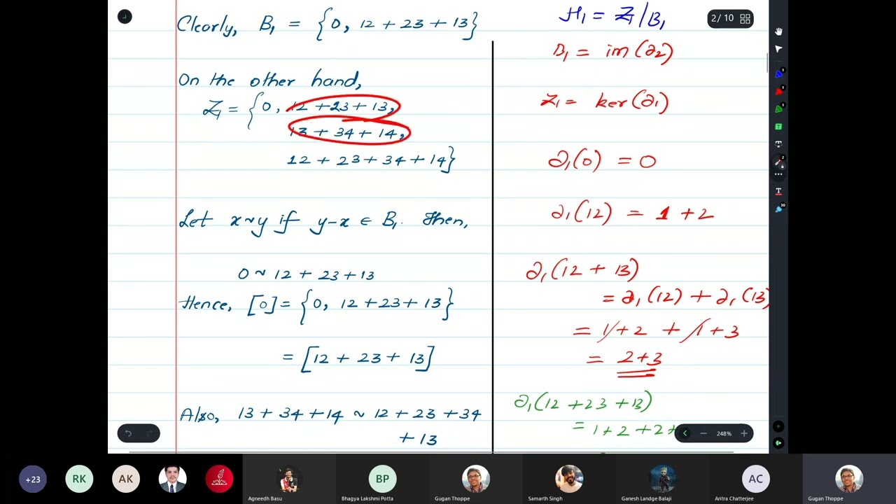
all right so this matrix is now reduced it's our reduced boundary matrix and from this reduced boundary matrix we can read off the persistent homology why is it reduced it's reduced because each lowest one in a in in any column is sort of in its own unique row and those lowest ones that are in their own unique rows those are called the pivots so here are the pivots of this reduced boundary matrix and it's these pivots that really sort of um determine the pairing that gives you persistent homology essentially when reducing the boundary matrix you're sort of changing dimension on the um area so you're sort of changing basis you're changing basis on the on the group of chains and you're changing basis to find a convenient basis to represent cycles and boundaries is what you're doing in the language of homology okay so i need to show you how to read off the persistence barcode from this matrix i'm going to label each persistence interval with the simplex whose birth whose appearance gives birth to that interval and with the simplex whose appearance uh kills off that interval so let's start with one dimensional homology in in purple the generators for homology are the cycles the things with zero boundary those are going to be our empty columns because you know these are things that when i take their boundary i get zero so when i have the sum of these four edges a b plus b c plus c d plus 80 when i take its boundary um i get zero so this is going to give birth to a one-dimensional feature okay so empty columns give births to features this one-dimensional feature appears at time three okay so it's going to be this bar how do i find when this feature dies well this feature first appeared um with edge cd so now i go to the row corresponding to cd and i ask is there a pivot in this row there is that tells me the death time of this feature this feature that was born at time three is now killed at time six okay and furthermore you can see the chain that filled in this feature the chain that filled in this feature was the sum of two triangles right this hole corresponding to four edges was killed when these two triangles filled in so there's a lot of geometry you can read off here's another empty column that also gives birth to a one-dimensional hole it's this one-dimensional hole that's born at time four okay and it's this triangle a b b c um ac and then ac was the edge whose appearance gave us this triangle so i look at the row corresponding to ac and i ask is there a pivot in this row there is and that pivot tells me when this feature dies it dies at time five so that's why this bar that was born with the edge ac dies with the triangle agency and again you see this hole is filled in by this triangle stepping back a moment um if you only want to describe the homology at this stage there's no reason you needed to use the square and the triangle to represent the two holes you could have used the two triangles but the persistent homology algorithm finds a consistent basis that works not only at this stage but also at all other stages for example including this stage where you need to have the square as one of your generators in this one-dimensional loop all right so these were the empty columns you know corresponding to edges that gave us one-dimensional holes let me also look at the empty columns corresponding to vertices which are going to give our zero dimensional persistent homology intervals okay so vertex a has an empty column it's going to give birth to this infinite interval when you look at the row corresponding to a there's no pivot in this row right you know this isn't a pivot because there's a lower one this isn't a pivot because this is there's a lower one so since there's no pivot in this row this feature is unpaired and it lives on forever here's another empty column b gives birth to a zero dimensional connected component we look at the row corresponding to b it has a pivot so this connected component that was born at b dies when this edge a b appears connecting it to something that had already appeared a so that gives this bar right here c is an interesting one you'll notice geometrically that c appears at the same time this edge appears so it shouldn't really give an interval of any length so we look at c it is an empty column okay so it does give birth to a zero dimensional feature but when we look at the row we see that there's a pivot that says that c was born at times two but it it this feature dies also at time two when this edge appears okay so this feature sort of is born and dies at the same time and that's why we don't draw a bar far for it and lastly let's get to this empty column corresponding to vertex d okay so it appears at scale two it's going to give us this bar i look at the row corresponding to d to find this pivot and and this pivot is telling me that that at time three there's an edge a d that appears connecting d to earlier stuff so that's why this bar that was born at time 2 dies at time 3.
all right so thanks so much for your time and attention i didn't give a full rigorous introduction to this algorithm but i i hoped to walk through it on an example so you get to see some of the moving parts and i hope to explain some of the geometric intuition that you should focus on when you're trying to learn and understand this algorithm thanks so much you
Up Next

82:15
Computing Persistent Homology: Lecture Tutorial With Examples
@utahsoccomputationaltopolo4135
3.3K views•2021-02-17

4:43
Elliptic Curve Cryptography Explained: ECC, ECDSA, ECDH
@PracticalNetworking
28.5K views•2024-10-21
5:04
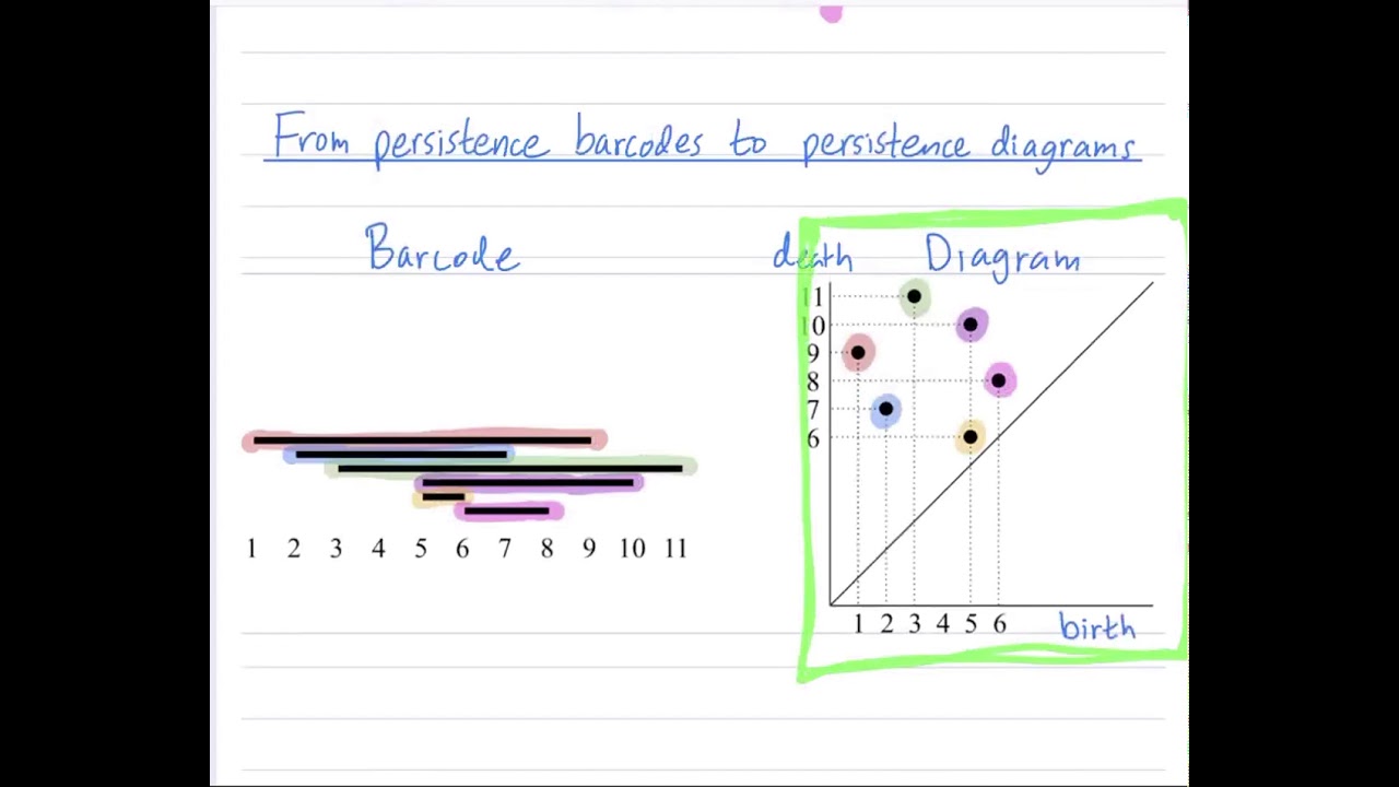
Persistence Barcodes vs Diagrams Explained | TDA Tutorial
@aatrn1
4.9K views•2021-02-18

6:00
The Mathematical Impossibility of Accurate World Maps
@Vox
23.3M views•2016-12-02
Related Study Plans & Knowledge Roadmaps
Structured learning paths in Mathematics
mathematics
Tensor Calculus: Vectors to Riemann Curvature
01Mathematical Foundations: Linear Algebra & Calculus
02Covectors, Dual Spaces, and Tensor Basics
03The Metric Tensor and Index Gymnastics
+ 2 more learning modules
40h5 modules
Explore Roadmap
mathematics
Gödel's Incompleteness: Logic, Proofs & Limits
01Introduction to Formal Systems & Hilbert's Dream
02Set Theory, Cardinality, and Cantor's Diagonal Argument
03Arithmetization and Gödel Numbering
+ 2 more learning modules
14h5 modules
Explore Roadmap
mathematics
Galois Theory: Fields, Groups & Solvability
01Foundations of Abstract Algebra: Groups & Fields
02Polynomials & Field Extensions
03Splitting Fields & Symmetries
+ 2 more learning modules
24h5 modules
Explore Roadmap
mathematics
Non-Euclidean Geometry: Models & Geodesics
01Euclid's Fifth Postulate and the Birth of New Geometries
02Hyperbolic Space and the Poincaré Disk Model
03Geodesics: Defining Straight Lines in Curved Spaces
+ 2 more learning modules
15h5 modules
Explore Roadmap