
















![#22 Machine learning Andrew Ng Tiếng Việt [Khóa 1, Tuần 2, Bài học 1]](https://i.ytimg.com/vi/M97tkKAqd9I/maxresdefault.jpg)









Persistent homology is computed by constructing a filtration of simplicial complexes from point cloud data, then performing column operations on boundary matrices to identify topological features (cycles that are not boundaries). The Mapper algorithm provides an interactive visualization of this process, showing how high-dimensional data can be decomposed into connected components and loops through a one-dimensional skeleton. The rank of the homology group captures the number of independent topological features (such as tunnels or loops) in the data, which can be used for downstream machine learning tasks like classification and regression.
Computing Persistent Homology: Lecture Tutorial With Examples
Added:Basic Simplicial Homology: Understanding simplicial complexes, chain complexes, boundary operators, and how classical homology groups are defined.
Linear Algebra and Matrix Reduction: Familiarity with vector spaces, matrix operations, and reduction algorithms similar to Gaussian elimination.
Concept of Filtrations: Grasping how a nested, growing sequence of topological spaces (complexes) is constructed over a changing scale parameter.
Abstract Algebra Basics: Familiarity with algebraic structures and field coefficients, particularly computing homology using coefficients in Z/2Z.
Persistence Diagrams and Barcodes: Learning how to interpret and analyze the birth-death representations of topological features across filtrations.
Stability Theorems in TDA: Exploring the theoretical guarantees that make persistent homology robust to noise, specifically using the bottleneck and Wasserstein distances.
Vectorization for Machine Learning: Converting persistent homology outputs into formats like Persistence Landscapes or Persistence Images for integration with ML models.
Multidimensional Persistence: Studying advanced mathematical frameworks where complexes are filtered by multiple parameters simultaneously.
Practical Application of Mapper: Applying the Mapper algorithm to perform topological data analysis, visualization, and clustering on complex, high-dimensional datasets.
3.3K views0likes1:22:15Original Release: 2021-02-17
all right yoja would you like to go ahead and share your screen yep all right so as i mentioned before uh you guys are a guest lecturer for today where he's going to spend um up to 10 minutes to talk about a tool that compute um mapper graphs on the fly so remember we spent quite a bit time discussing the mathematical foundation as well as application of a tool called uh mapper construction um and it's coming from rib graph and so on and there's several open source software out there and one of them is developed developed by yuja like she's a primary developer for that and it's called mapper interactive and i believe there's a in the chat window um yuja can you put a link to the software yes so yeah i've put the link to the chat window all right go ahead yeah and hi everyone i'm mio cha so here is the interface of this interactive tool and let's go to a simple example to see how these two works so first of all let's import these uh 3d horse data so this is the uh 3d point cloud data of like a horse so you can see the how this point cloud data looks like here and after importing this data set uh the system will show like all the columns you can use to uh build clustering so in this in this case you can both select more columns or delete some columns so here we just use the all three columns to do clustering and after that you can do some parameter adjustment of the clustering so let's do this and after i'm going to quickly intersect right those are the parameters that is used for um for the db scan algorithm so if you record there's multiple parameters associated with the mapper in this case you just software only care about the mappers mapper graph which is one dimensional skeleton of the mapper construction so when you think about what other parameters you need to specify um for the clustering you need to specify the parameter in this case if you choose db scan then you need to choose the parameter associated with db scan where epsilon is uh the size of the local neighborhood and mean sample is sort of the minimum density requirement for db scan and then you have parameters related to the number of intervals amount of overlap what is the filter function and because this is a visualization tool it's also you need to choose what is a color function all right go ahead yuja and after that you can choose your filter functions you can do either 1d mapper or 2d mapper and let's do the 1d mapper first so you can choose your filter functions through the drop down manual and here we just do the the average of the node values and you can also adjust the number of intervals and the rate of overlap here after that we can just compute the mapper so here is the result of this mapper graph but it's still a little bit hard to understand so let's do some coloring of the note first in this case the the y value represents the head of the the head value so if you look at here it means like from 0 to 0.8 and let's just coloring it of the head value and we can also size it use the same value so in this case you can see this very small yellow nose is actually represent the four feet of the horse because the feet is at the lowest head and this very large red nose is actually represent the head of this horse because the head is at the highest head in this case so it's showing the skeleton of this 3d horse and after that you can do some analysis based on the mapper graph we have for example we can do linear regression we can also do pca like to co compare the result of pca with our macro graph and you can also select some nodes to compare their average values of each column and to see like uh within each node which rows it contains you can also do like select the entire cluster or select the path as does the node the nodes are connected so i'm going to inject here quickly so what happened is um um one thing that we did not dive into detail when we were talking about macro construction is that if you're giving me a high dimensional point cloud you know if you think about the mapper algorithm it is a sort of a fancier clustering algorithm of this high dimensional point cloud and in a sense that is capturing how points are clustered and how those clusters are related with one another so one sort of downstream analysis you can play with the mapper graph or the macro construction is you can select subset of the high dimensional point cloud by selecting nodes in the macro graph so i could potentially just click on one node of the map graph and then apply things such as linear regression what you just demonstrated is there are multiple ways to select subsets of the macrograph for example you can select a particular branch by using the select path right yoja if you can demonstrate maybe you select one of the leg of the um yes if you select one of the leg right maybe this one yeah so you can select so in a sense that what what we can do is now if you select a subset of the data points you can look at the distribution of each dimension of points in each of the nodes that is involved in sort of this leg of the horse and then you can also apply things like linear uh linear regression okay so why is this interesting because part of this um if you think about linear regressor as a sort of as a model to feed the data if i apply a linear uh sort of regression for the entire point cloud usually what you're doing is you're trying to find a single hyperplane for the entire point cloud right but now if i'm actually sort of decompose my data point into subsets and apply sort of linear regression for each of those subsets then what you're doing is in some sense creating what's called a partition page a partition-based regression model or another way is a mixture of linear regressors so in a sense that you can decompose your data into subset subsections of perhaps in this case based on the mapper graph and apply linear regression for each of the partition right you kind of sort of study the trend of the data that is related to say a particular branch or particular area of my macrograph okay so that's something you can do essentially if you're if you have a topological summary of my high dimensional data using things like mapper graph then what i would like to do is to do downstream machine learning uh onto the entire point cloud or subset of the point cloud that is defined by the topological structure okay all right you just keep going yep and in particular if you selected a subset of nodes all the analysis will be based on the the selected nodes for example the the pca result will now be look like like one leg of this uh of the whole data point actually this looks like multiple legs yeah i don't know why it should be only like i think there's also part of the body remember you choose part of the body yeah yes yes like this part no but i also suspect that maybe your leg has i don't know a ring but it's interesting to look at why this is the case all right okay and should i also show uh real data yeah i would go i would go with the cancer data set okay yeah let's see sorry let's see which one is the this one okay so this data set is uh like a breast cancer data set um we will uh it contains like uh i think this desert is only contains a few number of genes and also like the uh whether this binary variable indicating like whether the patient is dead or alive and in this case we only use the genes to compute to do the clustering and then we go back to the to the uh parameter settings so we said epsilon equals 0.45 and main samples equals 2 and then we also also in this case we can do like 2d members so one of the uh like we can do one of the filter function let's do the even depth and we can and another maybe we just do like the l2 norm so the purpose of this uh of of our uh our goal of doing this data set is to identify the subset of patient uh so we are hoping to do some like uh to divide the entire data set into a few subgroups that like in this situation we we have these two disconnected clusters like one is for the the alive that alive patient and another is for the dead patient and maybe i will just use the size to do so we can we can like explore uh like what's the difference between each of these two groups maybe i will just show the result in our paper like to because this it is better than than this well the paper uses the entire data set than this smaller data set right but go ahead yeah so this is actually the result we have so we have like a few uh clusters that with the alive patient and a few clusters with the dead patient and we are identifying so i i believe like the the color function here is let me see well the left-hand side of the picture is uh is a label whether they survive or not of the cancer right yes yeah so i think the coloring function is like one of the genes so usually like if the if the value of this gene is uh relatively large that indicating the patient has high probability to be alive and if it is small it it is uh like more likely the patient is dead but we just identify this branch with a subset of patients that uh has this uh lower expression value of this gene but they still alive so we can do some more analysis within this subgroup all right okay all right so i think it's good uh to stop the demo here so um there is multiple other tools uh thank you yuja so there's multiple other tools that is used uh for um for sort of mapper and then they have or have sort of very different strengths um and so macro interactive is actually one of the newer tools that our our team has just developed and it has more of interactive capabilities and computing mapper graphs on the fly there's also some other tools also in the same category of open sourced mapper algorithm implementations that later on we might be exposed to some of those as well so okay so that's the first component of today's lecture the second component is actually i want to describe a little bit over and thank you yuja for for your time um my second component today is i would like to go over quickly uh the description of the first project which is just released uh so let me share the screen all right can folks see good all right so um i'm just going to describe this quickly and if you have some questions uh please ask now and this is release today oh it's released last night but it's today and it's going to do on march 4th uh so remember march the week following that is uh is where i would call the mental a break or sort of our not so official uh spring break in the sense that we don't have class on march 8th um but this is due before that so hopefully you can get this done and kind of have a relaxed week all right it's not very complicated in a sense that this is a project i would like to test your sort of understanding and your ability to compute persistent homology so the overview it has it's um it's it's a mini project meaning that the final score is 20 of your final grade um it has a few components to it the first part should be very easy um basically i would like you to compute barcodes slash persistent diagram of of several synthetic data sets okay so the software itself is called ripster if i have time today we'll go through a quick demo of how to get it installed and get it to run um but what it does is if you provide a point cloud and or if you provide a pairwise distance matrix it's going to compute the barcode for you okay so the first part is to compute barcodes for some synthetic data set and the second part is to compute the barcode for image dataset so i'm providing some sort of minimum guidelines to how exactly you're going to do for the part two because i would like to explore the data and the hope is that i'm kind of simulate a real world simulation uh that i don't give you a user manual for the new data set and you have some freedom to how you would like to explore it and and it's also part of a hack where i give you here is the open source package and you know maybe you need to modify the code maybe not depends on how you want to proceed maybe you have to write a module that does the data wrangling at the beginning okay which is exactly part two of this project so what you're going to do is you're going to record the persistent barcode in the form of a txt file so for a particular data set once you run it it's going to output and you're going to talk about the birth and death of each of the bar um you're going to provide a screenshot of your output and also you're going to provide source code um and i think faye has an announcement that for the project it's it's it's going to be submitted through grayscope but it's going to have two components one component is the pdf of your report report of the mini project and second part is a zipped file of your source code we do that because then she can directly comment based on your report so she can mark onto the pdf and so on right and um so ultimately your report is going to consist of the screenshots together with the pdf description and you are going to have the barcode and source code in a zip file and then they will make that clear over announcement on canvas to exactly the format she wants you to do for submitting through grayscale but if you look at sort of the pipeline for tda or tablature data analysis is you have some sort of data and in most cases what we have been talking about so far has been point cloud data um but you can also be graphs it could also be images in the second part in this project exact images and now what you're going to do is you're going to construct this filtration of simplicial complexes in the form of point cloud data especially for ripster the simplicial complex it's construct is actually a via taurus ribs complex which is something we described before and once you compute this filtration meaning that each of the simplex has an uh ordering attached to it you compute the persistent homology which comes out as a barcode representation from the ripster software um and of course once you have this barcode the downstream analysis is things like machine learning and visualization and so on and so forth so what is the data the first data is already for part one is some synthetic data set one is called octa one is called cylinder of course cylinder is pretty obvious because it's a point cloud sample from a cylinder octa i would like you to try to visualize a point called you know and see what it is but both of them has interesting dimension zero and dimension one homology okay so the second part of the data set is the mpeg-7 image dataset and here's a link to it and here's an example of this data set it's basically the silhouette of a bunch of shapes okay and what i would like to do is to figure out a way to compute the persistent homology of this image data set okay for the part one um you know i already provide you some synthetic data set and you can even play with more sensitive data set but the idea is i would like to for both of those data set there's a particular type of um persistence feature i would like to return um i would like you to return them um as sort of the bars in the barcode and i want you to compute for both of them dimension one persistence uh homology okay and you know give you a hint that octa is going to consider it contains four very large loops in their data set okay and then there are some very small loops also as well so in total octa contains eight loops in the data set for of course for a cylinder it at least have one loop because the tunnel of the cylinder so what i'm looking at is i'm looking for is basically a basic usage of the software ripster and to be able to export them in sort of a text file right so play with a synthetic data set the second part is that for this image set i would like to take 10 sample images one from each class and i would like to design what's called a filtration for each image i'll make that clear very soon and once you get the filtration you kind of want to represent this image maybe as a point cloud okay and you want to compute the barcode in dimension 0 and return the barcode again as a txt file so part of the second part require a bit of data processing meaning that what are the potential ways to construct a filtration remember the image oh well there's a compelling thing anyway there's a there's a there's a reference towards the end i'm going to update this file um there is a particular paper well there's first option is you have if you look at this point cloud right you have a silhouette of the shape so one way you can convert each of image to a point cloud is to just sample point at its boundary okay so basically try to extract the points that separate the black from the white pixel okay so you have a cell away point cloud and then you can compute sort of the persistent homology of this point cloud okay that's option number one which is slightly easier option but if you want to challenge yourself the second way to do this is to say okay i am not only going to well i mean the second way to do this is to say okay i have a point cloud but instead of computing a filtration using the point cloud directly i am going to put a height function on this point cloud okay so what do that mean i'm going to take sort of because it's a two-dimensional image i can take a height direction in a disk okay in a circle so meaning that i can define a height function that is say vertically and i couldn't define a function that is horizontally i can also define a height function that is forming 45 degree okay so for each of those height functions you can also construct a filtration of it and hopefully soon in not today's election later i'll tell you how that filtration is constructed it's very much based on what's called sub-level cell filtration basically i'm going to look at how the points grow as i'm i'm looking at all the points that is below a certain threshold of my height function but the high level picture is for giving a shape like this even in any of those point cloud or shape i'm going to take a collection of height direction defined in the point cloud for each of this height direction there is going to be a persistent diagram so now for each of the shape i'm going to get a collection of persistent diagrams okay that was a second option of course the third option which i haven't mentioned is instead of getting the silhouette of the points i can also convert this image to another point cloud which is only the point sampled from either the white region or the black region okay so that's another way to convert this to a point cloud representation i can just take this image and i can say okay i'm only going to sample points from the black background okay or i only sample points from the white uh foreground okay so that's another way to turn it into a point cloud and try to perform analysis okay and then last bit what people can do which is not very effective in this case because this is just a black and white image but if the image has sort of more color to it then you can treat the whole image as a scalar function and apply persistent homology to it but that's not recommended for this particular data set because it's only really if you're thinking about values is usually just have two values right let's say zero for white and one for black or other way around so there's only two scalar values so in a sense that if i just treat this image as a scalar function uh it's it in computing sub-level system this scanner function is not going to be very effective because it's not not a continuous function all right so okay so second part as i mentioned there's a reference here which is basically what's called deep learning with topological signature okay so if you actually look at this what i described earlier is basically taking different direction of a shape and computing the barcode it's actually what's called persistent homology transform it's a particular technique to say that okay if i want to characterize a shape instead of just looking at you know the behavior of the point cloud itself i want to look at the behavior of it with respect to a collection of function defined on it and happened to be the collection function i care about is all the direction i can model right so in 2d i have a direction surrounding a circle where i can kind of rotate my angle to define which direction i'm defining at the height of this of this shape and i'm going to get the persistent homology with respect to that direction in 3d if i have a 3d model then i'm going to sample it all sort of high direction that is sampled from a sphere and if i sample the argument under the persistent homology transform is that if actually there's a really interesting reconstruction problem surrounding it which is if i have a particular 3d model and i take enough directions to compute the persistent barcode if there's enough of those directions then i can argue i can reconstruct the original shape all right this is very similar to the idea that you know to do like sort of image reconstruction of sort of 3d model reconstruction from images so if i have a 3d model let's say my water bottle right and i go around with the different camera angles if i take enough angles of the camera to take a collection of images then there's argument that with all those 2d images i can reconstruct the 3d object this is actually similar but from the perspective of persistent homology the argument is if i take enough direction high direction to compute the persistent barcode and if i collect enough of them all those persistent barcode combined together it's going to recover my original point cloud of the shape okay so the second part like if you take this option you are basically looking at uh how do you actually you know apply this kind of thing to get a collection of signatures from those image things so if you want to challenge yourself to go with option number two then you want to read the paper which also come with the code okay so so in a sense that for the second part of the mini project i give you more options of how would you like to proceed with the image data set and and part of that is really rely on how do you process the image to turn into a form that is usable by say ripter or by the software purpose associated with uh with the deep learning paper what does that paper do actually once you get a 3d shape and you take all different direction you get the persistent diagram what they do is they use those persistent diagrams associated with the shape now each shape is associated with a collection of persistent diagram they are using that for shape classification okay so if you imagine in the small data set [Music] if you have this small data set here one option is to say if i expand this data set to a larger collection for example all sorts of images that is from you know i don't know the image of apple different apples or image of horse image of deer then the idea is can i use those persistent diagram for classification tasks okay so in some sense that this mini project is essentially the sort of pre-processing for downstream uh classification tasks and then you are using topological sort of persistent diagram as topological features that can be used as an input to downstream analysis okay all right any questions on the project okay all right uh yeah feel free to use piazza um to ask questions uh about the project and my recommendation is to start as soon as you can you know this is not a project you want to wait until the day it's due uh to start to start okay all right go ahead yeah i saw that ripster is a c plus plus um are we so are we to use c plus for so part of this part of so i believe if i if i remember correctly ripster does have a python interface i believe and maybe i'm wrong but you should correct me um most part of this project you can pretty much use ripster out of box you see what i mean however if you do end up having to modify it feel free to ask me or fade if you have any issues okay and in in some sense part one i'm a hundred percent sure you can just run rips or out of the box for part two once you have done so there are some coding you need to do for part two precisely how you pre-process the image data set to a format that ripster can take so that's pretty much you can state you you can pretty much avoid modification of rip source code does that make sense yeah that's kind of what i was asking about was just for the pre-processing step like can we use python or you can do pi sound right i would actually suggest python i think majority of people know more about python nowadays but uh but yeah so part of part two is a pre-processing stage and you can use any language you want right you just want to pre-process the image data into a form that is acceptable by ripster and do you care about like seeing that pre-processing script or can we just say okay yeah so so part of the yeah so as i know so far ripster has a python library but only include a subset of api that the actual ripster actually have yeah i mean yeah so so i would encourage people to look into that right yeah so yeah so i kind of remember it has a python interface but it might not have all the capabilities uh but yeah but if you want to stay pure with python it's doable um yeah so so as part of submission what we're asking for is you're going to submit a report that includes screenshot description of what you did and also the source code and usually um for all the project is that you have to provide enough detail that faye and i can reproduce your result meaning that your code has to be executable i mean in some sense that you know if it's pi cell we can run our machine right so in a sense that uh we are looking for code that is usable i mean it doesn't have to be like you know uh production quality but it has to be enough for us to repeat reproduce your results that would be the requirement for the code submission i know there's a few of you who is not a cs background um so feel free to reach out uh to get help from me and fee but i would say for this first mini project a lot of it is about using existing tools there's a question in the chat can you hear me yes i can hear you it's not very loud but go ahead oh there's a question that chat asking about the um the colored image that you talked about so to clarify option four for colored image processing did you mean sort of like so with rgb oh no no so that that is just my comment it's not related to this project for this particular mini project i specify you're going to download the image from the mpg mpeg-7 image data set which is black and white images i'm saying that if you actually want to apply the same type of framework to color images then you can have sort of rgb images and then you can process them slightly differently than you do with the black and white images but that's not part of the mini project one yeah i think i think that um sun hoon knows that it's just he's asking is this sort of like r squared plus g squared plus b squared for each pixel and then somehow accumulated function values there's few ways to do it right you basically want to convert a colored image into a scalar field and there's multiple ways to do it depends on sort of which channel do you care most does that make sense thank you okay all right any other questions for the project all right so usually according to our class syllabus the project is due on the on the day that is stated and it's due before the class starts um but start earlier and start asking questions and especially for those who don't have um you know this will be a good starting point uh for you to get familiar with some of those tools all right so the other part today you know i'm going to is a little bit out of order but let me since we're talking about tools i want to mention that um you know there's a lot of open source tools out there so the ones that uh you have seen today mapper interactive is one tool that compute micrograph the ripster is another is another tool open source tool that computes um a persistent diagram but based on viator's ribs filtration of the point cloud there's a history of open source tools in computational topology and anthropology analysis over and over the past five years i would say there is actually really a large collection of them uh here is an incomplete list um there is java plex which i believe is one of those java implementations of computing personal homology there's tdar which is a our implementation um and especially for people in statistics and math people like to use the use r so tdar is our package for topological data analysis especially persistent homology computation but it also contains some other statistical tools inside there's a dionysus which is one of those earlier tools also implemented in uh cc plus for a persistent homology computation it also contains some other form of persistent homology including zigzag and so on there's goodie a diva and fat those are gudi is an open source tool that contains a lot of collections of typological guitar analysis tools including persistent homology but it's also include things like discord i believe uh it's also include uh other tools that is go beyond simplicial compasses like what we call qubit simplices which is a different type of filtration of point cloud data um and it's actually supported by a really large group um diva and fat are the tools to compute personal homology uh in a scalable way i mean to be fair mapper interactive also contains a few speed up that we have to apply to uh point cloud data with a large scale when i say large scale i'm talking about one million points okay so one million points and beyond if you play with ripster as part of your project one i'm saying that's going to come back and you're going to realize when you are doing that project is that depends on how many points you sample from the image it might significantly impact uh the computation your your laptop computer might run out of outer memory uh in some sense within a few thousand points a part of that is because when you're constructing the same position complex um even with a few thousand points your simplest complex might have one million elements um and uh you know later in this lecture we're going to go over a very simple example of computer persistent homology by hand and you can see that even with three points in my data set i'm going to have a matrix that is you know up to uh up to a quite large and also that in the worst case scenario the persistent homology algorithm is n-cubed meaning that n is a number of simplices and the algorithm runs in n-cubed worst case uh which is not a very scalable thing in the worst case however in practice if you have n simplices the the typical practical of a practical runtime is roughly linear in the number of simplices but again even if you have one million simplices the wrong time is still going to suffer all right so those tools are the ones that is based on essentially uh scalable computations so i want to go through here of course this is going to scoot up my link oh okay hold on one second so there's two links i provided over there oh i think there's a space hopefully this is not okay so here is uh an incomplete collection done by one of my a friend and uh collaborator uh talking about all the open source software options okay and and there is the mapper algorithm mapper interactive isn't there yet because it's just the most recent tool there is a first one which is ayasti which is their tool uh sort of commercial grid tool using mapper computation their skeet kit tda which is part of a kepler mapper which include kepler mapper that include again a sort of python slash html version of of constructing a mapper from point cloud data uh there's tda mapper and there's a python mapper which is one of those earlier tools in computing mapper persistent homology you have a really long list of computation we just mentioned ripster which is what you're going to use for the first project but there's also all this uh a different tool set that um that uh that that include personal homology computation uh one thing i do want to mention is due to tda this part this is also one of this newer package that is developed by folks at epfl and then it also contains quite a bit of capabilities not just persistent homology but also include mapper implementation as well um so perseus right perseus right here this is the one that is fairly scalable and of course the one that is very scalable um is the distributed version of person's homology computation which is difficult okay so uh so yeah so there is also some vectorization which is something we're going to talk later down the road is um you know we kind of had a small taste of of how topological data analysis interface interface with machine learning down the road we're going to talk about approaches that takes a persistent diagram and convert it into vectors such that it's easier to be used as input to machine learning algorithms such as you know svm and uh and the neural networks okay so there's multiple ways of converting a persistent diagram into a vectorized form and depends on what you want to make use of there are certain forms where you convert to it's much easier for what's called kernel based machine learning methods so we're going to describe that later down the road is how do you convert persistent homology information into vector and then there's of course other computations for example later on when we talk about the distances between persistent diagram um is what's called hera so if i have persistent diagram one thing to do is to compute the distances between persistent diagram right if i'm using persistent diagram as a feature for things like classification or regression i need to be able to measure distances between those feature vectors represented as persistent diagram then there's distance measures between them for example bottleneck distance and washington distance so the idea is actually going to compute those distance fast and hera is a package that help compute those distances between persistent diagram all right okay so that's that for some of the open source packages and later on you're going to see some of this and what you just saw earlier is the mapper interactive demo by yuja and then there is a paper that goes with it if you want to um you know kind of look at more data sets and or examples and then the data set that it described in the paper is also part of the distribution of the software so you should you should try to sort of play with those high dimensional data set and to kind of get familiar uh with the mapper algorithm the other one i do want to mention right um this was an earlier tool that is using uh sort of our implementation of of a topological data analysis and then there is information on how to in store and there are also tutorials how to play with it if you are a fan of r but part of this is that this is just a screenshot of it on the right-hand side the left-hand side is a code but right hand side what you see is i have two point cloud one a big circle and a small circle with point called sample from those two circles and what you see is the persistent diagram in the bottom remember you know what i described the barcode it's talk about birth time and death time of each bar the persistent diagram is alternative way of encoding it where the black points here corresponding to the zero dimensional persistent homology where the circle also rectangle red rectangle corresponding to one-dimensional persistent homology so there is sort of two points in this diagram two sort of rig uh sorry not rectangle triangle in this diagram that corresponding to two of those circles right so those are one dimensional homological features uh that is counter so of course depends on the distance of this points to the diagonal it tells you how persistent it is which corresponding to how sort of significant or important that feature is you see those two uh triangles that is off the diagonal the one that is closer to a diagonal corresponding to the lower left corner of the small circle versus other one corresponding to the big circle so in a way that this loop is corresponding to this and this loop corresponding to this okay so this is just a quick demo of of how how would you see from you know the interface of tdar which is one of those tools that compute personal homology okay any questions okay if there's no question let's get back to a little bit left over when we are talking about computing persistent homology what i want to do today is at least to go over one example of computing persistent homology by hand all right so what do i want to do so let's do a quick recall over what we learned from last lecture all right so let's start with the hey do you want to take a break i wanted to say this oh yes yes let's take a quick break uh let's take uh five minutes break we'll come back at 1003 okay and feel free to ask questions if you have any okay so let's uh resume i actually had a question about the the last graph that you showed before it [Music] which one it would be impossible for anything to be under that curve right which graph are we talking about um the last one um with the homology it was in your other set of slides sorry this one yeah yeah okay so so you you're saying um how close things are to the line basically shows their life but just so i'm reading this right it's impossible for anything to be under that line um in the current construction we have uh uh no um but a lot of answer in this direction is not absolute because what we're in this lecture was actually in the semester we're going to mostly talking about the sort of the classic sublevel set filtration or distance filtration and in most cases the sort of the points are basically in this upper left triangular area because what happened is that for each of the point in here it has a burst time and a death time and usually burst time is smaller or equal to this time right you have to board first before you die however depends on how people doing the filtration there's something called extended uh persistent homology and what that looks at is sort of looking at the filtration for subluxial filtration and the super levels filtration and so on and then in that case that gives rise to a persistent diagram which has point in here but that's not something we're going to cover uh in the lecture but it's actually described in the textbook okay all right thank you all right so let's get back to um the important definitions um so so again i was warn you that those are sort of algebraic topology uh first chapter in like a crash course uh but we're going to sort of spending a few more lectures to go over a few examples hopefully this will become clear um so there's a concept we went through last lecture what is a cycle right a cycle is a one that has is a a a one cycle is a one chain with empty boundary so if i take a boundary of it it's zero okay so there is this sort of what is a kernel of a function the kernel of a function is basically everything that mapped to zero so if i want to have a picture of it if this is a function going from its domain to its range then there is a subset of element let's say in the domain that mapped to zero okay let's say this is my subset let's say a a is a subset of my domain that through this function it all mapped to zero then what we say is a is equal to the kernel of the function so the notation here when i say it's a kernel of a function it means that it mapped to zero through the function it's part of the points in the domain that mapped to zero that means it's a kernel now there's a definition of an image now remember i have again you know let's say my my my domain let's say for this example is integer my code domain is integer remember i said my function is 2 times this right so i say okay so if i have point one point two where does it map to one is going to map to two in here two is going to map to four in here and so on so forth so basically everything that is mapped in here through the function f going from the input to the output meaning that my this set here let's say it's b b is a subset of the integer and b is the image of my function meaning that it's all the possible output uh from the input right so i take all the possible input and map it to a possible so it's all possible how to say values uh my function can take uh in the range of the function or co-domain of the function so in this particular example if my input if my domain and codomin are both uh integers then the image from this function as i defined are all the even uh integers right or the even numbers are in my image okay so this is kernel image but by definition remember a cycle is a one with empty boundary so because of this definition if i take the boundary of its equal to zero that means it's a kernel of of of this boundary map and the the p boundary is a chain who is the boundary of the p plus one chain so a one boundary is a boundary of a two chain so a one boundary is the boundary of a linear combination of triangles and by definition they are the image of the previous map and because of this right remember i say that the boundary so boundary is an image a boundary group is an image of the boundary map and a cycle group is a kernel of the boundary map so that's become the picture here for example if i focus on the yellow bp which is the p dimensional boundary group it is the image of cfp is an image of the p plus one chain group right that's the definition and now if i look at for example z of p well let me erase this if i focus on the zfp remember the definition this is all the kernel of the boundary map so because it all matched to zero right so now what's happening is the homology group right here is the sort of the quotient operation or module operation between z of p and b of p what does that mean it's sort of it's a homology in this case let's say p is equal to one i care about the loops one-dimensional homology the one-dimensional homology are the ones who are psych who are um how to say they are cycle group right remember they are the p dimensional cycles but they are not boundaries so this quotient or module operation is to say that i care about uh element in my one dimensional homology group if it is it is so h1 is equal to z1 modular p1 it says that it's a one dimensional homology group if it is a one-dimensional cycle but not a boundary so when you take the modular operation is to say that i'm going to ignore part of my elements in this group that is boundary so what does this mean if i just focus on z1 sorry if i'm just focusing on dimension one homology to be z1 modular b1 so i want to say it's one cycle that's not a boundary so from an english language perspective what does that mean so first of all it has to be a one cycle so let's say i have a one cycle that is a linear combination of edges so i have one two plus one three plus three four plus two four okay so this is this is a one cycle because if i take the boundary of this this is equal to zero okay so this is a one cycle but the question is that is this a boundary so it's not a boundary because there does not exist a linear combination that is c2 c2 means that it does not exist a linear combination of triangles such that the boundary of this linear combination of triangle is equal to the current one dimensional cycle so it's not in a sense it's not a boundary of a linear combination of triangles however now if i give a second example if my chain is 1 2 plus 1 3 plus 2 3 we know you know in this case c so in this particular case let me go back this this first example c is in z1 because it's uh um it's it's a linear combination it's a linear combination of edges and it is a cycle but then it's not uh it's not a boundary so what that means that means c is part of this homology group so what is the picture looks like is that this yellow linear combination bunked up tunnel where does it where's the tunnel it's right here because there's an empty space that corresponding to the one-dimensional tunnel or one-dimensional homology group now if i use the same example except for a different chain where i have linear combination of one two two three one three now what happened is that this chain is z one which means it is a boundary oh sorry it's a it's a cycle because if i take the boundary of it is equal to zero right so that's the first part and now it also means that there exists a c prime which is equal to the triangle one two three that's part of c2 such that the boundary of c prime is equal to c so what does this mean this means there exists a linear combination of triangle in this case just one triangle whose boundary is my current chain so that means this implies my chain is part of a boundary also so this means that this because c is in z1 and c is in e1 this implies c is not a dimension one homology and from the picture it's obvious it's because it's not bounding a tunnel because the tunnel is already filled by a triangle okay so again you know there's this picture here but the most important part is really in if i were going to picture what does my homology looks like what i'm getting is you know my p dimensional homology group are the ones who are part of the p dimensional cycle group modulate the p dimensional boundary group which is basically corresponding to the cycles which are not boundaries okay so those corresponding to essentially those tunnels we're describing about but this applies to any dimension so far i have been using dimension one because it's easier to explain so if i were going to have a picture view anything that is in the cycle group but not in the boundary group is my homology group so this is sort of this yellow region now corresponding to uh sort of the hormone the elements in my homology group all right so so once we have this concept there's what's called the rank of it in some sense the rank captures how many independent um tunnels do i have uh okay so how many independent elements do i have so part of this is that if i have a chain let's see the first chain which is one two plus two four plus three four plus one three i have another chain which is two three plus three four plus um two three three four and two four okay so let's see the first chain is all those yellow edges and then the second chain is all these pink edges my point is that those two one dimensional chain of both both of them both c1 and c2 are part of the dimension one homology group meaning that they are both bounding a tunnel right one dimensional homology are tunnels they both bound to tunnels but even by just looking at this picture you see that they are bounding the same tunnel which means that they are actually not independent from each other so in this particular example right the ring well actually i already wrote here the rank of the dimensional homology is actually uh one because there's only one independent cycle or sorry tunnel in this space okay but of course if i give you a different space you know this is something you want to think about and we'll come back to this example okay this is my more complicated space in this particular example it's going to tell you when you compute the rank of the dimension one homology this is example where rank of dimensional homogeneous group is equal to two meaning that there's two independent tunnels there there's this one and then there's this one okay but of course there's multiple uh linear combination of edges that describe this tunnel same thing as what i just described you can have you know this one described in the first tunnel and this one describing the second tunnel and then you can have this one describing the linear combination of both tunnels okay those are all elements in my dimension one homology group so with the remaining time today um so so again we're going to come back to it um the rank of a group is sort of the generators and we're hopefully going to give more examples of it but this is sort of the mathematical notation of it idea is i want to look at independent tunnels in my dimensional homology but what i would like to do is to go over one example of computing persistent homology there's three examples of what i'm just going to go over for one of them okay so because this helps with your understanding of how to use rips or down the road so here is an example of a simplicial complex that has three vertices and three edges and there's no triangle and i'm going to label the three vertices to be vertex one vertex two vertex three and the three edges to be h4h5h6 that's it and then the numbering of it also corresponds to what i call the filtration meaning that when does those vertices and edges appear so i would say vertex 1 up here at time 1 vertex 2 appear at time 2 vertex 3 up here times 3.
edge 4 appear at time 4. h5 appear h time 5 h6 up here at time 6. and then this is exactly this is what's called the boundary matrices which is basically each of the column is a simplex ordered by the time they appear each row are the vertices and simple vertices and edges again ordered by the time they appear and then there is going to be an entry of a one if a particular vertex is a boundary of of the edge so if a particular rows are part of the boundary of a particular column so this is a very simple uh filtration as i see is what's called filtration is if you have a collection of simplices that they appear in some ordering and that is my filtration of course there's additional that my boundary of a simplex has to show up before the simplex itself but in this case you know all the vertices show up before the edges okay so the first of all i'm going to look at the boundary of vertices well there are zero boundaries so there's nothing in the entry of my of my of my matrix and here i'm going to look at what is a boundary so what is the boundary of my edge 4 can anyone help me what is the boundary of my edge it's one two vertex exactly it should be the vertex 1 vertex 2.
i'm using this quotation mark just to say that those are labels also on there so because a boundary of 4 is 1 2 so you have an entry of 1 and an entry of 1 right here and then the boundary of h5 is right the vertex 2 and vertex 3 so there's corresponding one in those entries same thing the boundary of the last one the boundary of 6 is 1 and three that is my boundary matrix now what i would like to compute is if i go through this filtration right the vertex appear and disappear when does homology dimension one homology up here uh when does dimension zero homology appear okay so before we go through the computation i want to go through this example by itself okay i'm going to use a space on the left corner what is my time so i'm going to add uh what is the sequence of my thing it's one one two three four five six okay so if i'm thinking about my time at time the first at time 1 vertex 1 shows up at time 2 vertex 2 shows up at times 3 vertex 3 shows up okay and then at time 4 the edge shows up the h4 shows up h5 shows up h6 shows up okay so this is what i call the filtration that every single time there are some simplex that shows up in the same position complex so now my question for you if i'm looking at zero dimensional homology okay when are the components born you know without computation i just want to look at this filtration okay when does component bore equals one two three yeah so there's a component born at time one there's a component born in time two there's a component born times three so you're right when do they die four five and six exactly so of course now you have to make a decision you know like which one do i die right so if there's an edge connecting the component one two remember the rule is the youngest rule so the youngest one dies first okay so between one and two it makes one one two merge that means the component two merge into component one then the two component dies so this is two four okay now at time five the component represented by one is merged with the component represented by three but three is the younger one so i say three dies okay and then the component that is com represented by the vertex one never dies so this is a dimension one homolog dimensions uh dimension zero uh persistent homology okay now what is homology in dimension one when does a loop appear a tunnel appear six six exactly when does it disappear sorry go ahead do you see it never exactly this are now my barcode okay because the dimension zero barcode tells me there's component die at two disappear at four border two disappear at four there's a component boy and three disappeared five there's a component that never dies and then in dimension one person's homology is there there's a there's a tunnel that is born at time six uh it never dies because i never put a triangle in there to kill it off so but how do i do this through a matrix operation okay so i want to now do a matrix operation and i'm going to do this example for today and then we're going to go through a few more examples next time but feel free to try to challenge yourself with the first examples the the the operation of persistent homologous computation can be completely encoded by column operations and the column operation goes from left to right so i start from left okay i'm just going to operate on this boundary matrix here i start from the first column it's empty i don't have to do anything i don't have to do anything i don't have to do anything now i'm going to finally arrive at a non-empty column and what i'm going to do is looking at the lowest one so the lowest one right of this column is the one i just put in a square and i'm going to look to the left of it to see if there's any other one there if there's no such one i don't do anything i'm done okay now i'm going to the next column i'm going to look at the lowest one the lowest one is right there this entry and i'm going to look to the left there's nothing conflicting with it i'm done the last column is this one so this is where things become interesting i look at the lowest one and i look to the left and what's happening is that there is a one also to the left of it so what i'm going to do is i'm going to add this column to the current column because i detected you know a 1 there so i'm going to add the column 5 to column 6. so what do i do in term of operation one say i'm going to add column five to column six i'm going to add basically move the value from five to six and add them so i basically add one to this here and another one to here but then it's one plus one that is equal to zero all right so basically now what i have is once i add five the fifth column to the sixth column i have cancelled out this lowest one right here so i get a i end up getting one one zero in this column now i'm going to check again the lowest value of this okay but because you know i already operated over five so for the time being i'm going to ignore the fifth column but i'm still going to look to the left and because of this i see that okay i have one one but the fourth column also has a lowest one right that is conflicting with the current one so i'm going to add four to it so the fourth column is added to my current column and again it's one plus one equal to zero one plus one equal to zero so at the end of this you get this matrix where the after i added both column 4 and column 5 to this column 6 you got all 0 in that column okay and then this is what i call reduced matrix now so i have now reduced my boundary matrix to this new matrix and what i'm claiming is everything i just talked about in terms of the barcode is included by this matrix okay what did that mean now let's look at their dimensional feature zero dimensional feature are born um so so what do you do here is first of all you look at the ones that is enclosed by once okay so those lowest one that i didn't touch the lowest one in those rectangles are the ones corresponding to finite features meaning that the feature that has a burst time and a finite burst time and finite this time so the row the row index is its first time the column index is is this time so what did this mean this means there's a feature that is born at two and die and four there's a feature that is born at three and diamond five this corresponding to precisely the two zero dimensional feature right two four three five as i went through this process here now i care about the features that is probably born but never dies right those corresponding to the empty columns okay so well of course empty columns you know some of them is already paired so you want to ignore them so there's four empty columns there's the first column second color third column and the last column but the but the second column and the third column is already paired so you kind of ignore them right because they are born at this time but they died at time four and time five so yeah so in some sense they are already encoded as this burst time but then you see there's two more columns the first empty column and then the last empty column the corresponding to birth of a component one it never dies and compo birth and time six and never dies right and then of course the first three of them are zero dimensional feature and the last one is one dimensional feature okay so that will conclude what i want to talk about today to compute persistent homology it's basically boiled down to column operation over matrices and next lecture we're going to go over two more examples but how does this work uh for for your first project you provide a point cloud and then you provide a filtration which is the ordering of the simplest as the columns one ripster well actually what ripster does is it takes a point cloud first and construct this filtration based on rip's filtration and then it's going to compute the barcode as what i just did by doing those column operations okay of course there's some optimization they did in the code to make it fast but this is really the naive algorithm to compute versus homology okay any questions uh yeah i had a question so uh why is this not considered a triangle oh why is not a triangle yeah because this is this this simplistic complex only contains three vertices and three edges there's no triangle in there oh this space so this space as i drew is not the same as this space those are two different simplest accomplices oh i see oh okay okay right that makes sense okay thank you but you can actually push yourself right let's say i want to do the persistent homology of this space what's going to happen i'm going to add a column in my column matrix to b7 and 7 is my triangle and the boundary of the triangle the boundary of my triangle so i'm going to add a column and a row is going to be four five six okay i believe this is my next example well my next example is a little bit more complicated do i have another one no yeah so so this will be an example you can play with which is if i add the triangle in here what is going to happen what's going to happen is that it's going to have a tunnel that is a tunnel that is born at six and it's going to die at seven when the triangle comes back okay all right i'm going to start streaming and people can ask me more questions
Up Next
5:04
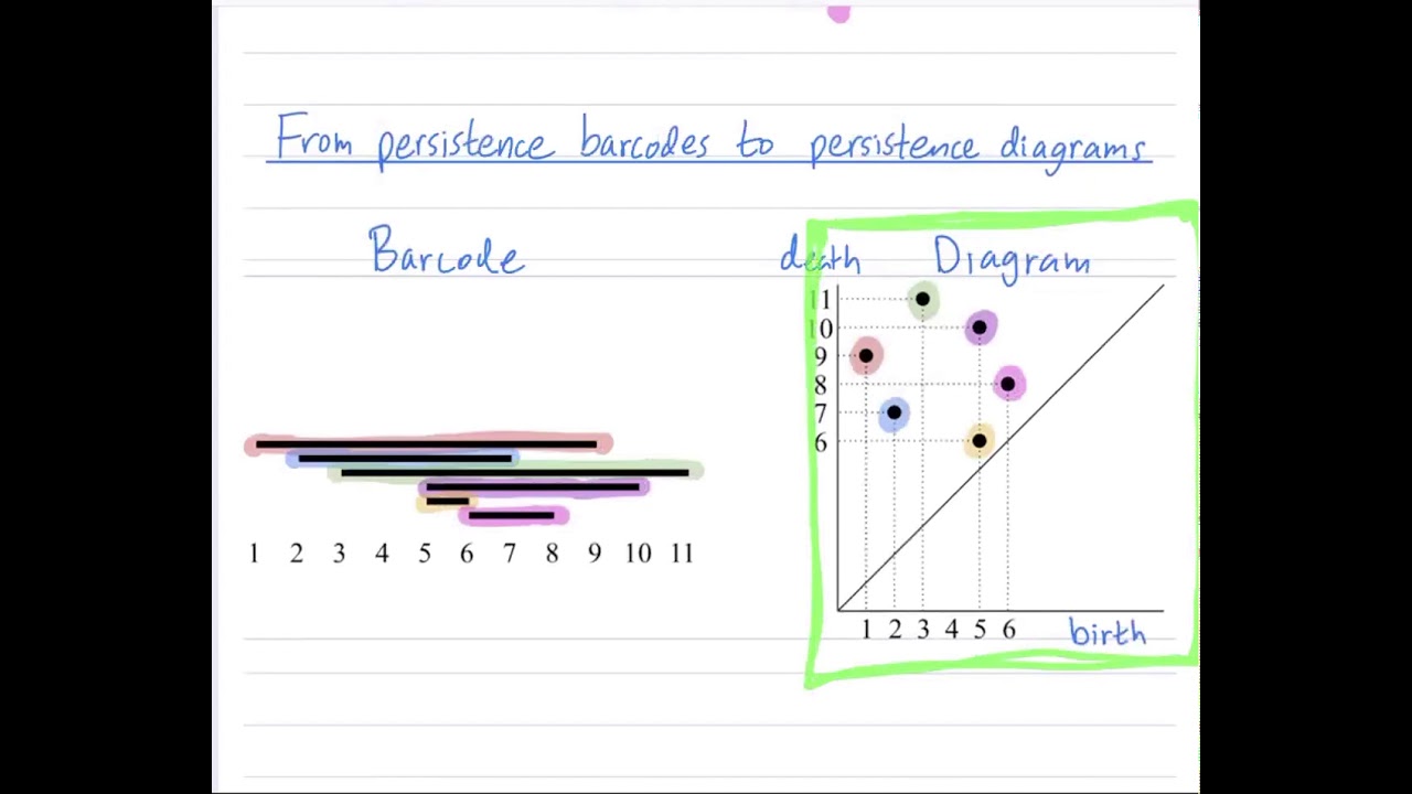
Persistence Barcodes vs Diagrams Explained | TDA Tutorial
@aatrn1
4.9K views•2021-02-18

4:43
Elliptic Curve Cryptography Explained: ECC, ECDSA, ECDH
@PracticalNetworking
28.5K views•2024-10-21

10:44
Fourier Series Introduction: The Big Idea Explained
@DrTrefor
387K views•2021-05-03

6:00
The Mathematical Impossibility of Accurate World Maps
@Vox
23.3M views•2016-12-02
Related Study Plans & Knowledge Roadmaps
Structured learning paths in Mathematics
mathematics
Tensor Calculus: Vectors to Riemann Curvature
01Mathematical Foundations: Linear Algebra & Calculus
02Covectors, Dual Spaces, and Tensor Basics
03The Metric Tensor and Index Gymnastics
+ 2 more learning modules
40h5 modules
Explore Roadmap
mathematics
Gödel's Incompleteness: Logic, Proofs & Limits
01Introduction to Formal Systems & Hilbert's Dream
02Set Theory, Cardinality, and Cantor's Diagonal Argument
03Arithmetization and Gödel Numbering
+ 2 more learning modules
14h5 modules
Explore Roadmap
mathematics
Galois Theory: Fields, Groups & Solvability
01Foundations of Abstract Algebra: Groups & Fields
02Polynomials & Field Extensions
03Splitting Fields & Symmetries
+ 2 more learning modules
24h5 modules
Explore Roadmap
mathematics
Non-Euclidean Geometry: Models & Geodesics
01Euclid's Fifth Postulate and the Birth of New Geometries
02Hyperbolic Space and the Poincaré Disk Model
03Geodesics: Defining Straight Lines in Curved Spaces
+ 2 more learning modules
15h5 modules
Explore Roadmap