The link budget equation (P_tx - P_rx - margin = path loss) uses the path loss formula PL = 20 log₁₀(4πd₀f/c) + 10n log₁₀(d/d₀), where d₀ is the reference distance (typically 1 meter), f is the operating frequency, c is the speed of light, and n is the path loss exponent that varies by environment (corridors, open areas, rooms, or between floors). This formula allows engineers to calculate the maximum communication distance for a given transmit power, receive power, and system margin.
Understanding Path Loss Exponent in Indoor Propagation Models
Added:Deep Dive
Basic principles of electromagnetic wave propagation and Free-Space Path Loss (FSPL).
![Free Space Loss [FSL] - Entender las pérdidas de espacio libre](https://i.ytimg.com/vi_webp/DnsKmQ_hd34/maxresdefault.webp)
Free Space Loss [FSL] - Entender las pérdidas de espacio libre
9.4K
Free space path loss (FSPL) is the fundamental signal attenuation caused by electromagnetic wave spreading through free space. The standard formula is FSPL(dB) = 92.4 + 20 × log₁₀(frequency in GHz) + 20 × log₁₀(distance in km), or 32.4 when frequency is in MHz. The underlying geometric principle is the inverse square law: when distance doubles, the wavefront area quadruples, reducing energy density by a factor of four. This explains why signal strength decreases with distance. The received signal strength is directly proportional to antenna effective area, meaning doubling distance requires four times the antenna area to maintain the same received signal. Every 3 dB change represents a doubling or halving of power, providing a quick mental calculation method. FSPL is distinct from attenuation, which accounts for environmental losses rather than geometric spreading.
Click to watch →

L-4 Free Space Propagation Model, Wireless Channel Propagation Mobile Network Planning ,Optimization
719
The Free Space Path Loss (FSPL) combines power density and antenna gain formulas. The general form is: FSPL = (4π × Distance × Frequency)² / (Transmitter Power × Transmitter Antenna Gain × Receiver Antenna Gain). An alternative form uses antenna gain relationships: FSPL = (Transmitter Power × Transmitter Antenna Gain × Receiver Antenna Gain) / (4π × Distance² × Frequency²). These formulas show that received power decreases with the square of distance and frequency, which is fundamental to wireless propagation physics.
Click to watch →

ENLACES - 1ra Parte - Sistemas de telecomunicaciones
81.8K
Free space path loss (FSPL) is the reduction in signal strength as electromagnetic waves propagate through space. RF signals spread spherically from the source, meaning only a portion of transmitted energy can be captured by the receiving antenna while the rest disperses into surrounding space. The FSPL equation is: FSPL = (4πdF/c)², where d is distance, F is frequency, and c is the speed of light (3×10⁸ m/s). This shows path loss increases with the square of both distance and frequency. For practical calculations, the equation is converted to decibels: FSPL(dB) = 20log₁₀(4πdF/c). This logarithmic form simplifies calculations and enables easier comparison of different link scenarios.
Click to watch →
Antenna And Wave Propagation | Vaibhav Jain | Unit-3 | Electronics Engineering | AKTU
7.6K
Free space path loss (FSPL) is the loss in signal strength due to propagation through free space: FSPL = (4πr/λ)². It represents the reduction in power density as the wave spreads out over the spherical surface area at distance r.
Click to watch →

Cálculo Radioenlace
11.1K
The Free Space Path Loss (FSPL) formula calculates the major portion of total attenuation caused by electromagnetic wave propagation effects in the air. The formula is: FSPL = 20 log₁₀(distance in km) + 20 log₁₀(frequency in MHz) + 32.45. The distance must be in kilometers, frequency in megahertz, and the result is in decibels (dB). The constant 32.45 represents the values for an isotropic antenna.
Click to watch →
Deep Dive
Proficiency with logarithmic mathematics and decibel (dB/dBm) calculations used in signal power measurements.

Data Communication mid exam segment 2 part 2 CSE-3525
196
The decibel formula dB = 10 × log₁₀(P_received / P_sent) measures signal power changes. When power is reduced to half (0.5 times), dB = -3 dB indicating attenuation. When power increases 10 times, dB = +10 dB indicating amplification. The dBm formula dBm = 10 × log₁₀(P_milliwatts) measures power in milliwatts. For -30 dBm, P = 10^(-30/10) = 0.001 mW. These logarithmic scales simplify large power ratio comparisons.
Click to watch →

#329 QO-100 How Do We Get 20 Watts Output on 2.4GHz Wi-Fi
70.9K
To achieve 20 watts (43 dBm) output on 2.4 GHz, a 20 dB attenuator is needed to protect measurement equipment, and the required amplifier gain is calculated by subtracting the source power (1 dBm) from the target power (43 dBm), resulting in 42 dB of amplification needed; this demonstrates how dB/dBm logarithmic calculations simplify power measurements in RF systems.
Click to watch →
![[HAM] Kurs Krótkofalarski #3 Modulacja i detekcja](https://i.ytimg.com/vi/NcmU-nrxx9w/maxresdefault.jpg)
[HAM] Kurs Krótkofalarski #3 Modulacja i detekcja
1.2K
A logarithm answers: to what power must the base be raised to obtain a number? For example, log₁₀(100) = 2 because 10² = 100. The decibel (dB) is a logarithmic unit for expressing signal ratios. For power: dB = 10 × log₁₀(P₂/P₁). For voltage: dB = 20 × log₁₀(V₂/V₁). Key shortcuts: +10 dB = ×10 power, +3 dB = ×2 power. dBm references 1 milliwatt, dBW references 1 watt.
Click to watch →

#291 External antennas and ESP32 Long-Range mode
235K
The decibel scale is logarithmic: 0 dB = 1, 10 dB = 10 times, 20 dB = 100 times, -10 dB = 0.1 times, -20 dB = 0.01 times. For power measurements (dBm), 0 dBm equals 1 milliwatt. Therefore, 20 dBm equals 100 milliwatts, and -20 dBm equals 0.01 milliwatts. This logarithmic scale makes large ratios easier to express and calculate.
Click to watch →
CHUYÊN ĐỀ VẬT LÍ 11- BÀI 6 : SUY GIẢM TÍN HIỆU KẾT NỐI TRI THỨC
9.7K
The decibel (dB) measures signal attenuation or gain as a ratio: dB = 10 × log₁₀(P₂/P₁). Positive dB indicates gain, negative dB indicates loss. dBm measures absolute power: dBm = 10 × log₁₀(P/1mW), using 1mW as reference. For example, 0 dBm = 1mW, +10 dBm = 10mW. The attenuation coefficient (dB/km) represents loss per unit length. To calculate received power: P₂ = P₁ × 10^(L_total/10), where L_total = α × distance. For example, with α = 0.3 dB/km and distance = 5 km, total attenuation = 1.5 dB. If input power = 2 mW, received power = 2 × 10^(-1.5/10) = 1.416 mW. These logarithmic units enable convenient comparison of signal levels across different scales.
Click to watch →
Deep Dive
Fundamental concepts of wireless communications, including carrier frequency, wavelength, transmitter power, and receiver sensitivity.

LoRaWAN 101
1.3K
This section establishes the core physics governing wireless communication range. Three key concepts are explained: Transmission Power (TxP) is the power accumulated and radiated by the transmitter; Path Loss is the signal attenuation that increases with distance as electromagnetic waves travel through a medium; Receiver Sensitivity is the minimum power level at which a receiver can successfully decode signals. The received power equals transmission power minus path loss. When received power falls below receiver sensitivity, communication fails. dBm (decibels relative to one milliwatt) is introduced as the standard unit for measuring power in wireless systems, converting very small power values into manageable numbers for calculations.
Click to watch →

Calculo Zona de Fresnel - Enlace de Rádio P01
3.3K
This segment covers fundamental concepts in wireless communications including the relationship between frequency and wavelength (wavelength = speed of light / frequency), where 2.4 GHz corresponds to 7.9 meters wavelength. The instructor demonstrates calculating power in dBm using logarithmic formulas (dBm = 10 × log₁₀(power in milliwatts)), showing how 250 mW converts to approximately 23.98 dBm. The segment also introduces the 5 GHz frequency band as an alternative to 2.4 GHz, discussing different propagation characteristics and interference patterns between frequency bands.
Click to watch →

Radio Frequencies, Bands, Modes and Bandwidth Explained.
131.3K
This comprehensive section covers the foundational concepts of radio communication. Frequency measures how many times per second electrical current switches polarity, expressed in Hertz (Hz)—88 MHz equals 88 million cycles per second. Wavelength is the distance between signal crests, calculated as 300 divided by frequency in MHz, and radio bands are often named by their approximate wavelength (e.g., 3.5 MHz = 80-meter band). Three primary modulation techniques are explained: Amplitude Modulation (AM) varies signal power according to audio input, Frequency Modulation (FM) varies frequency, and Single Side Band (SSB) removes the carrier and one sideband to concentrate all power into a single sideband for greater range. Bandwidth measures signal spectrum width—FM uses ~12.5 kHz while SSB uses ~3 kHz. Continuous Wave (CW) transmits a pure tone at ~600 Hz with only ~30 Hz bandwidth, making it the most efficient mode for long-distance communications.
Click to watch →

Introducción a ondas y frecuencias wireless (inalámbricas) - Curso de redes
23K
Frequency measures cycles per second, with units including Hz, kHz (1,000 Hz), MHz (1 million Hz), and GHz (1 billion Hz). Electromagnetic waves travel at 300,000 km/s (speed of light), creating an inverse relationship between frequency and wavelength: higher frequency means shorter wavelength. Antenna size is directly related to frequency—higher frequencies require smaller antennas, while lower frequencies need larger ones. Higher frequencies enable faster data transfer rates but shorter range, while lower frequencies provide longer range but slower speeds. This trade-off between data rate and range is fundamental to wireless communication system design.
Click to watch →
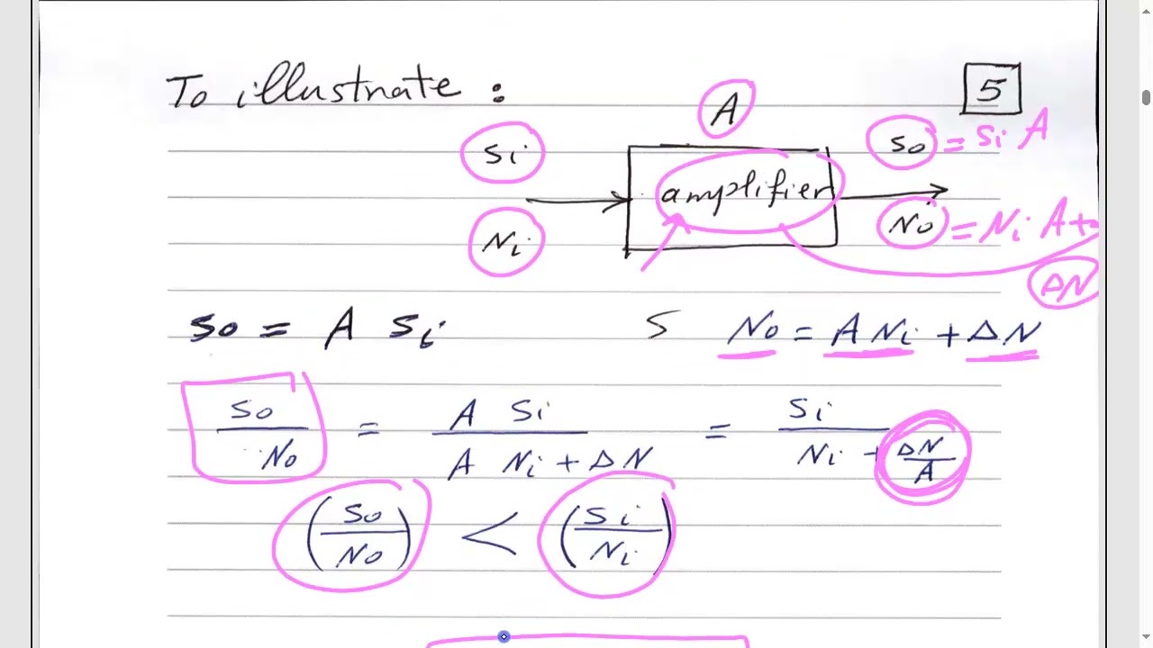
Lect 1 part a
924
In wireless communication, power is measured using logarithmic units dBW (reference: 1 watt) and dBm (reference: 1 milliwatt), where dBm = 10 × log₁₀(Power in watts / 1 milliwatt). Receiver sensitivity, the minimum power a receiver can detect, is calculated as: Sensitivity (dBm) = Noise Floor (dBm) + Carrier-to-Noise Ratio (dB), where Noise Floor (dBm) = -174 dBm + 10 × log₁₀(Bandwidth in Hz). The free space path loss model states that received power is proportional to transmit power and inversely proportional to the square of both distance and frequency, making higher frequencies suitable for shorter distances with higher data rates, while lower frequencies are better for longer-range communication.
Click to watch →
Deep Dive
Introduction to wave-obstacle interactions such as reflection, diffraction, scattering, and absorption.

PAES | Física | Resumen Ondas Electromagnéticas
6.8K
Absorption occurs when waves become trapped inside objects. For light, white light contains all colors; objects appear colored because they absorb all colors except the one they reflect. Black objects absorb more radiation and heat up more, while white objects reflect more radiation. Diffraction is the ability of waves to bend around obstacles and spread out when passing through openings. Interference is the interaction between two waves, which can be constructive (reinforcing each other) or destructive (canceling each other out). After interaction, each wave continues unchanged in its original direction.
Click to watch →

Physical Science Wave Interactions
2.5K
Wave interference occurs when two or more waves of the same frequency combine, with constructive interference (crests meeting crests or troughs meeting troughs) producing larger waves and destructive interference (crests meeting troughs) producing smaller or canceled waves; waves interact with each other through reflection (bouncing off surfaces, following the law of reflection where angle of incidence equals angle of reflection), refraction (bending when changing media due to speed changes, bending toward the normal when entering slower media and away when entering faster media), and diffraction (bending around obstacles); wave absorption converts wave energy into thermal energy, with thermal conductors transferring energy quickly and insulators slowly, reaching thermal equilibrium when absorbed and emitted energy are equal.
Click to watch →
![IGCSE Physics [Syllabus 3.1] Wave properties](https://i.ytimg.com/vi/xobSuCkaiU8/maxresdefault.jpg)
IGCSE Physics [Syllabus 3.1] Wave properties
97K
Waves interact with boundaries and obstacles through three primary phenomena. Reflection bounces waves off surfaces without changing frequency, speed, or wavelength—only direction changes. Refraction occurs when waves enter media of different densities, altering speed, direction, and wavelength while preserving frequency. Diffraction causes waves to spread out through narrow gaps or around barriers, with effect magnitude depending on wavelength-to-gap size ratio. These interactions explain diverse wave behaviors in nature and technology.
Click to watch →

Waves Interactions, Absorption, Transmision, Reflection. Physics Class Review.
293
Waves interact with matter and each other through five main mechanisms: (1) Absorption occurs when a wave transfers its energy to a material, causing the material's molecules to vibrate and reducing the wave's energy; (2) Transmission occurs when a wave passes through a material without losing much energy; (3) Reflection occurs when a wave bounces off a surface and changes direction; (4) Refraction occurs when a wave changes direction as it changes speed when moving from one medium to another, such as light bending when passing from air to water; (5) Diffraction occurs when a wave bends around an object or spreads out from an opening, like sound waves spreading through a doorway. Additionally, when two or more waves overlap, they combine according to the principle of superposition, resulting in either constructive interference (increased amplitude) or destructive interference (decreased amplitude). The law of reflection states that the angle of incidence equals the angle of reflection when waves bounce off boundaries.
Click to watch →

MRCOG Part 1 Exam Preparation Topic- Biophysics - Dr Preeti Poghe
1.7K
Ultrasound waves interact with tissues through five mechanisms: (1) Reflection occurs when waves reach an interface between media and return to the original medium; (2) Refraction is when waves pass through an interface into another medium; (3) Diffraction is the bending of waves around obstacles comparable to their wavelength; (4) Scattering is the combination of irregular reflection, refraction, and diffraction causing waves to spread in multiple directions; (5) Absorption is the conversion of sound energy into heat as waves travel through tissue.
Click to watch →
Prerequisite Knowledge
- Concept 01Basic principles of electromagnetic wave propagation and Free-Space Path Loss (FSPL).
- Concept 02Proficiency with logarithmic mathematics and decibel (dB/dBm) calculations used in signal power measurements.
- Concept 03Fundamental concepts of wireless communications, including carrier frequency, wavelength, transmitter power, and receiver sensitivity.
- Concept 04Introduction to wave-obstacle interactions such as reflection, diffraction, scattering, and absorption.
Subsequent Learning
- Step 01Log-normal shadowing models, which incorporate statistical variation to account for environmental clutter.
- Step 02Advanced multi-wall and multi-floor indoor propagation models, such as the Motley-Keenan model and ITU-R recommendations.
- Step 03Indoor positioning and localization algorithms that utilize Received Signal Strength Indication (RSSI) and trilateration.
- Step 04Practical RF site surveying, network planning, and link budget design for high-density indoor Wi-Fi and 5G networks.
Path Loss
Link Eq
Solve d
Path Loss
0:00Playing Section
- 1
Explains the common formula for average path loss at distance d.
- 2
Defines key parameters like reference distance, frequency, and light speed.
- 3
Discusses how the path loss exponent varies with indoor environments.
Deterministic Ray Tracing and Site-Specific Modeling
While the log-distance path loss model relying on a static Path Loss Exponent (PLE) offers a simple, computationally cheap method to estimate indoor signal attenuation, critics argue it is highly inaccurate for complex, real-world indoor environments. This limitation has driven the adoption of deterministic ray tracing and site-specific physical modeling. Unlike empirical PLE models, which average environmental complexities into a single statistical exponent, deterministic models use detailed 3D layouts of a building to simulate how radio waves physically interact with specific obstacles through reflection, diffraction, and transmission. Opponents of simple PLE-based models point out that indoor spaces suffer from severe multipath fading, dynamic human movement, and non-line-of-sight conditions that a single static exponent cannot reliably capture. Consequently, for high-precision applications like indoor localization, Wi-Fi planning, or 5G/6G deployment, engineers increasingly reject simplistic PLE calculations in favor of computationally intensive ray-tracing simulations or machine-learning-based fingerprinting.
Deep Dive
Log-normal shadowing models, which incorporate statistical variation to account for environmental clutter.

01 Multipath Effect - Model of Received Signal
342
Shadowing accounts for additional signal attenuation caused by obstacles between transmitter and receiver, such as buildings or terrain. It is modeled by multiplying the path loss result by a random variable expressed as 10^(ζ/10), where ζ follows a Gaussian distribution with zero mean and variance σ². When powers are measured in decibels, shadowing becomes an additive random variable, making it convenient for analysis.
Click to watch →

Log Normal Shadowing Model | Indoor Propagation Model | Wireless Communication
638
The Log-Normal Shadowing Model is an indoor propagation model that addresses the limitation of the Log-Distance Path Loss Model by accounting for random shadowing effects caused by obstacles between transmitter and receiver. The model expresses path loss as PL = PL₀ + 10n log(d/d₀) + Xσ, where Xσ is a zero-mean Gaussian random variable with standard deviation σ (both in dB), which compensates for random shadowing effects that result from changes in the degree of obstruction between the transmitter and receiver. The values of n and σ are determined from empirical data.
Click to watch →
Wireless mobile communication lecture no 10, Log normal shadowing path loss model, MKS
444
The log-normal shadowing model addresses the limitations of the basic log-distance path loss model by incorporating environmental randomness. The model recognizes that path loss at any distance D follows a random distribution described by a log-normal distribution in dB around the mean path loss. The random variable X_n representing shadowing is zero-mean Gaussian distributed in dB with standard deviation σ (also in dB). The complete model equation is: PR(dB) = PT(dB) - [PL₀ + 10n log₁₀(d/d₀) + X], where X ~ N(0, σ²). This framework enables statistical prediction of received power levels for arbitrary locations in communication system design and analysis. Parameters n and σ are estimated from measured data using least squares minimization of mean square error across multiple locations, while the reference path loss PL₀ is determined from close-in measurements or free-space calculations.
Click to watch →

Mod-01 Lec-37 Hata Model and Log Normal Shadowing
11K
This section addresses the random nature of wireless signal propagation beyond deterministic path loss models. Log normal shadowing describes random variations in received signal strength caused by large-scale obstructions such as buildings and walls. Unlike deterministic path loss, shadowing represents statistical variation due to the random clutter environment, making received signal strength a random variable. The random dB deviation about median path loss follows a Gaussian distribution with zero mean and variance σ². Since deviations are expressed in dB (logarithmic scale) and relate logarithmically to received power, this distribution is termed log-normal. The observed path loss equals median path loss plus a log-normal shadowing factor, enabling engineers to quantify coverage reliability in wireless networks.
Click to watch →
![[KUOCW] 고영채 이동통신공학(140310)](https://i.ytimg.com/vi/rrEjF_xy2UQ/sddefault.jpg)
[KUOCW] 고영채 이동통신공학(140310)
2.8K
Shadowing causes received signal power to vary around a mean value, following a log-normal distribution. When expressed in dB (logarithmic scale), shadowing appears as a Gaussian (normal) distribution. The path loss exponent (n) describes how rapidly signal power decreases with distance: free space (n=2), suburban (n=2.7-3.5), urban (n=3.5-4.0), dense urban (n=4.0-5.0). Higher values indicate more severe path loss due to obstacles. The complete log-normal shadowing model in dB is: PL(d) = PL(d₀) + 10n × log₁₀(d/d₀) + Xσ, where Xσ is a Gaussian random variable with zero mean and standard deviation σ (typically 3-12 dB). This model captures both deterministic path loss and random shadowing effect.
Click to watch →
Deep Dive
Advanced multi-wall and multi-floor indoor propagation models, such as the Motley-Keenan model and ITU-R recommendations.

Projeto e análise de enlaces indoor 2/2
117
This comprehensive section covers six propagation models for indoor wireless environments: Free Space Model (6 dB per distance doubling), Logarithmic Distance Variation Model (n=2.5-5), COST 231 Indoor Model (drywall 3.4 dB, brick 6.9 dB, floor loss 20-22 dB), ITU Indoor Model (Xs=7-14 dB random variable), and TATA Model (lw wall attenuation, floor loss factor). Model validation through measurements shows significant variation between predictions and actual values due to environmental specificity. The relationship between signal-to-noise ratio and channel capacity is emphasized as fundamental for reliable wireless communication.
Click to watch →

Capacitación HTZ communications parte 2
591
HTC Communications supports multiple propagation models including: (1) Free space path loss (Friis equation); (2) ITU-R P.525 for diffraction; (3) ITU-R P.525 for area attenuation; (4) ITU-R P.525 for standard area attenuation. The selection of propagation model significantly impacts simulation results, especially in urban environments where diffraction and reflection are important. The software allows configuring which phenomena to include in the simulation (diffraction, reflection, scattering, etc.).
Click to watch →
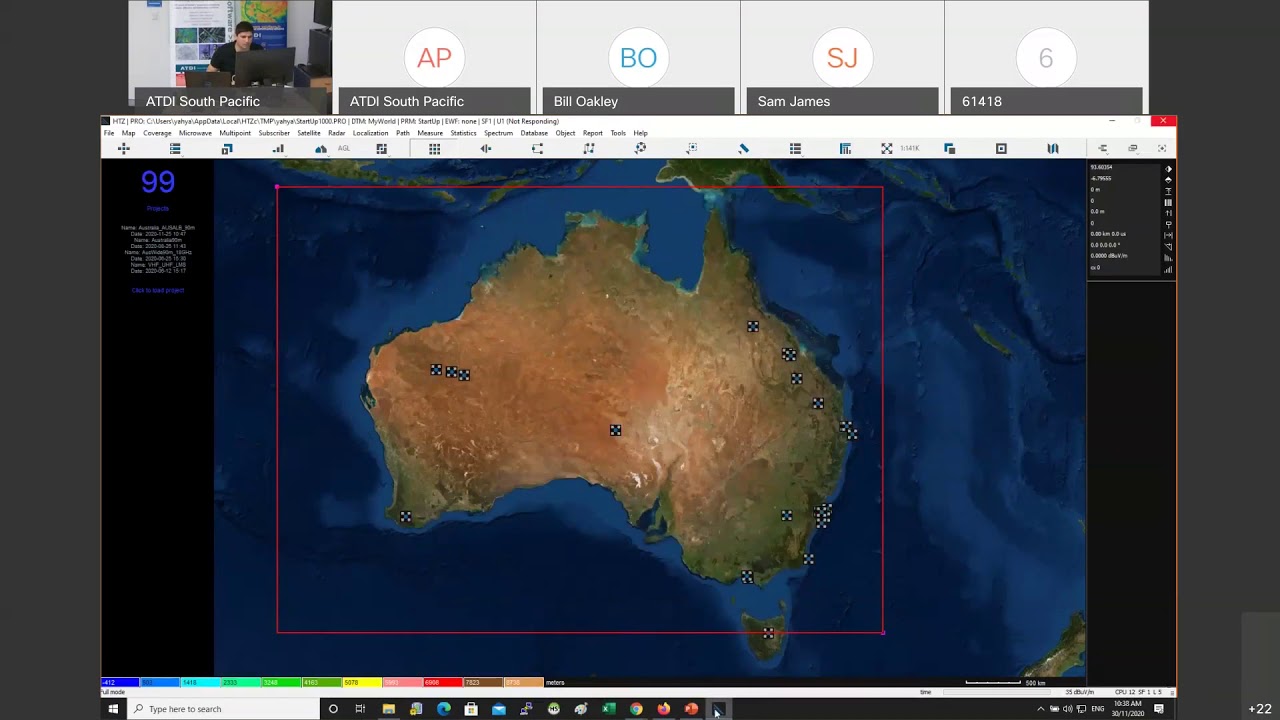
AWL area boundary contour analysis – the case of 28 GHz GSONGSO FSS
301
For AWL analysis in Australia, ITU-R 526-14 (deterministic propagation model using delta-Bolton method for diffraction) is the minimum required propagation model. Version 11 and 15 are available. Users can compare results using free space propagation (no diffraction or clutter effects) versus ITU-R 526-14 with and without clutter effects. Free space is useful for initial visualization but ITU-R 526-14 provides realistic terrain and clutter effects.
Click to watch →
WIRELESS & MOBILE COMMUNICATION LECTURE 08 ''Wireless Channel Modeling'' By Ms. Renu Sharma, AKGEC
3.2K
Propagation models are categorized based on environment type: Outdoor models include Okumura-Hata model for urban areas, COST-Hata model for suburban areas, and Hata model for open/rural areas. Indoor models include log-distance path loss model and ITU model for indoor attenuation. The choice of model depends on whether the application is for outdoor or indoor use, and whether the environment is urban, suburban, or rural. Rural environments have low population density and no high-rise buildings between transmitter and receiver.
Click to watch →
UNIT-2 :: WCN :: Indoor Propagation Models
494
Indoor propagation models describe how radio signals behave within buildings, differing from outdoor mobile radio channels due to shorter distances (typically meters rather than kilometers) and complex building structures including walls, floors, partitions, windows, and doors made of various materials like concrete, glass, and wood. These models account for factors such as building layout, number of windows and doors, room configurations, and partition losses that affect signal strength and quality. Common indoor propagation models include the Log-Distance Path Loss Model and Point-to-Multipoint models, which help predict signal behavior for designing indoor wireless communication systems like Wi-Fi and Bluetooth networks.
Click to watch →
Deep Dive
Indoor positioning and localization algorithms that utilize Received Signal Strength Indication (RSSI) and trilateration.
![Conception d'un système de positionnement local - local positioning system [FRENCH]](https://i.ytimg.com/vi/ATfyOr_ZPXA/hqdefault.jpg)
Conception d'un système de positionnement local - local positioning system [FRENCH]
114
A local positioning system determines the position of a tag within a limited indoor area by measuring the Received Signal Strength Indicator (RSSI) between the tag and multiple beacons, then applying trilateration to calculate the tag's coordinates by solving the intersection of circles defined by the measured distances from each beacon.
Click to watch →

EAI AISCOVID conference 2020 | COVID-19 AI-assisted Solutions & Smart Cities Biomed Applications
116
This research presents an empirical study of trilateration and clustering for indoor localization and behavior prediction. Indoor localization is the process of obtaining a device or user's location in an indoor environment, achieved through trilateration using RSSI (Received Signal Strength Indicator), Angle of Arrival, and Time of Arrival. Applications include healthcare (identifying activity patterns for depression and dementia detection), disaster management (rescuing people from indoor environments), and retail (presenting targeted advertisements). The system uses ESP32 devices as stations that receive BLE beacons and filter scan data. Bluejump beacons are used as tracked objects with battery life lasting up to 300 days. RSSI-based localization estimates distance using received signal strength and transmission power. The system was tested in Santa Clara University's indoor environment divided into corridor, lecture hall, and sitting area, achieving 73% accuracy after data preprocessing.
Click to watch →

SubPos - A "Dataless" Wi-Fi Positioning System
32.6K
Trilateration is the mathematical method used to determine position based on distances from multiple reference points. Unlike triangulation which uses angles, trilateration creates circles around each reference point with radii equal to calculated distances. The intersection of these circles determines the client's position. Using Received Signal Strength Indicator (RSSI), a path loss model can estimate distance, enabling position calculation through trilateration algorithms.
Click to watch →

EYE on NPI – XPLR-AOA Direction Finding and Indoor Positioning Explorer Kit #EYEonNPI #DigiKey
2.6K
Received Signal Strength Indicator (RSSI) measures how strong a wireless signal is at a particular location. Since signal strength decreases geometrically with distance from a transmitter, multiple receivers can use RSSI values to triangulate an object's position. However, this method has significant limitations: it only works reliably within 3-4 meters, suffers from signal reflections off walls and objects causing multipath interference, and cannot distinguish between direct and reflected signals.
Click to watch →

Wi-Fi positioning system
1.5K
RSSI localization techniques measure signal strength from a client device to multiple access points and combine this information with a propagation model to determine distances between the client and access points. Trilateration techniques then calculate the estimated client position relative to known access point positions. While one of the cheapest and easiest methods to implement, RSSI localization suffers from poor accuracy because RSSI measurements fluctuate according to environmental changes or multipath fading effects.
Click to watch →
Deep Dive
Practical RF site surveying, network planning, and link budget design for high-density indoor Wi-Fi and 5G networks.

Network Planning (part - 1) | Skill-Lync | Workshop
217
Effective site surveys collect multiple critical inputs: nearest points of connectivity for routing signals, area coverage assessment for determining tower requirements and budget, existing infrastructure analysis including landlord negotiations, population density evaluation correlated with throughput demand, existing network analysis for frequency coordination, and terrain/vegetation assessment for signal loss considerations. Link budget analysis calculates maximum communication distance (cell radius) between towers and users, determining whether a single tower can serve intended users and establishing coverage boundaries. This fundamental communication system technique applies to any wireless technology.
Click to watch →

Lesson 07.3-Understanding Predictive Site Surveys
1K
This section covers the essential concepts for wireless network planning and analysis. Decibel (dB) is a logarithmic unit that makes large power differences manageable. Link budget sums all gains and losses to ensure sufficient receive signal strength for signal recovery. Fade margin provides a buffer (typically 2-3 dB) for RF environment fluctuations caused by moving people and changing conditions. At 2.4 GHz and 5 GHz bands, signals reflect more than they are absorbed, enabling communication without direct line of sight. Network planning must account for the device with the weakest receiver sensitivity, typically IP phones. These principles enable accurate prediction of coverage and data rates.
Click to watch →

🎙️ Porta 443 | Omada by TP-Link
2.3K
Proper network dimensioning is critical because Wi-Fi operates on the electromagnetic spectrum and can cause interference when improperly deployed. Under-dimensioned networks have coverage gaps, while over-dimensioned networks cause interference and retransmission issues. The 2.4 GHz band has only three non-overlapping channels, making proper placement essential. Site surveys consist of three phases: predictive surveys model coverage based on floor plans and building materials; passive surveys identify existing interference sources; active surveys verify performance after implementation. Access points should be placed close to coverage areas with minimal obstructions, avoiding placement behind columns or in enclosed spaces.
Click to watch →

Wi-Fi at Large Public Venues | Ekahau Webinar
1.6K
Effective high-density Wi-Fi design follows a systematic five-step lifecycle process: (1) Site survey and assessment - gathering environmental data and interviewing stakeholders; (2) Requirements gathering - determining bandwidth needs and supported applications; (3) Design phase - calculating cell sizes and antenna selection based on consumption rates; (4) Validation - testing through AP-on-stick surveys and predictive modeling; (5) Deployment and optimization. Critical success factors include understanding client device consumption rates (80-95% utilization), performing passive spectrum surveys, and validating assumptions through physical testing. The methodology emphasizes that garbage-in-garbage-out applies to RF design, requiring comprehensive data collection before engineering decisions.
Click to watch →
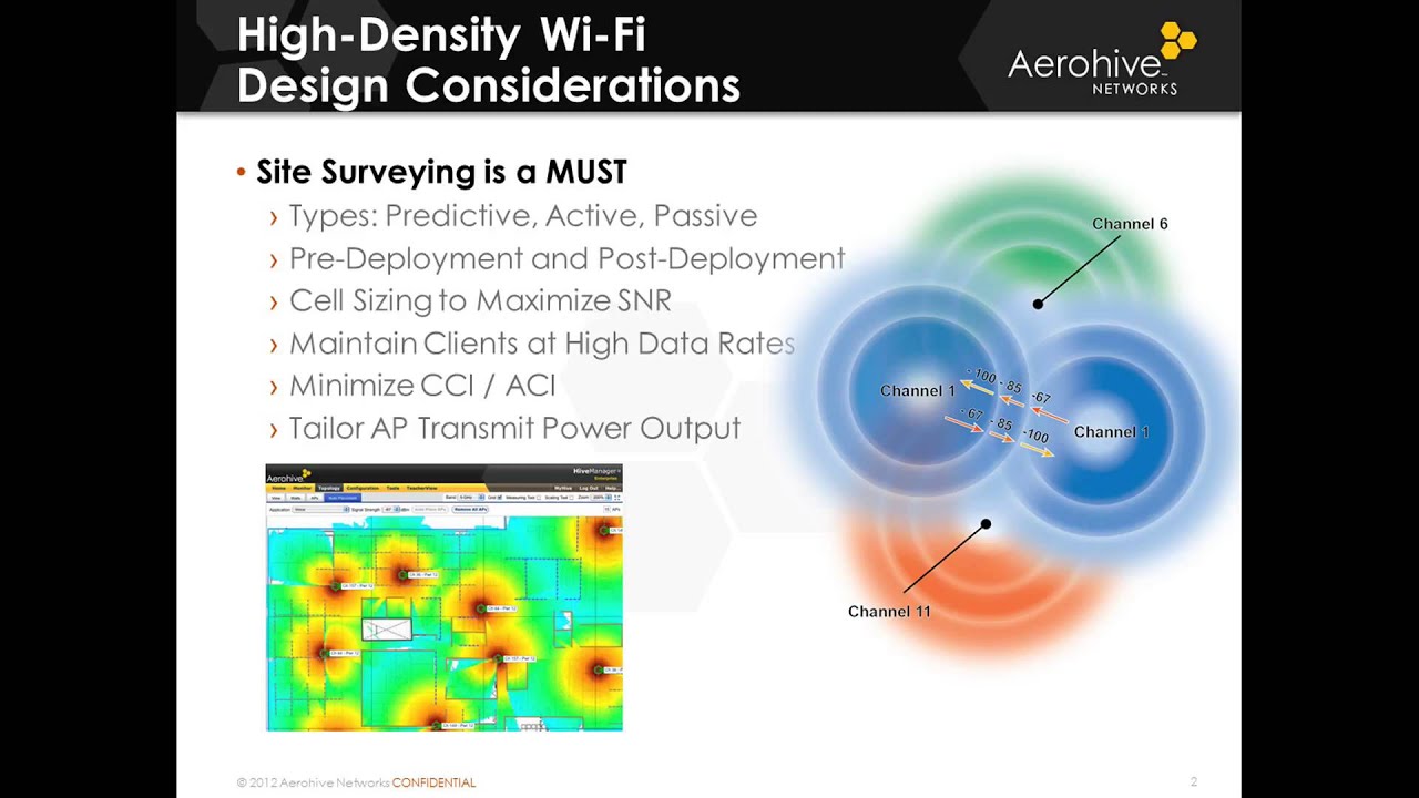
High-Density Wi-Fi Design Part 2 - RF Planning
20.3K
High-density Wi-Fi network design requires leveraging the 5 GHz band for greater channel capacity, using primarily 20 MHz channels with non-adjacent channel assignments to minimize interference, conducting thorough site surveys, implementing appropriate cell sizing with -67 dBm signal levels and -85 dBm interference thresholds, optimizing transmit power for bi-directional links, utilizing building obstructions to enable channel reuse, and strategically positioning access points with appropriate antenna selection to maximize capacity while minimizing co-channel interference.
Click to watch →
Path Loss
Link Eq
Solve d
Path Loss
0:00- 1
Explains the common formula for average path loss at distance d.
- 2
Defines key parameters like reference distance, frequency, and light speed.
- 3
Discusses how the path loss exponent varies with indoor environments.
Deterministic Ray Tracing and Site-Specific Modeling
While the log-distance path loss model relying on a static Path Loss Exponent (PLE) offers a simple, computationally cheap method to estimate indoor signal attenuation, critics argue it is highly inaccurate for complex, real-world indoor environments. This limitation has driven the adoption of deterministic ray tracing and site-specific physical modeling. Unlike empirical PLE models, which average environmental complexities into a single statistical exponent, deterministic models use detailed 3D layouts of a building to simulate how radio waves physically interact with specific obstacles through reflection, diffraction, and transmission. Opponents of simple PLE-based models point out that indoor spaces suffer from severe multipath fading, dynamic human movement, and non-line-of-sight conditions that a single static exponent cannot reliably capture. Consequently, for high-precision applications like indoor localization, Wi-Fi planning, or 5G/6G deployment, engineers increasingly reject simplistic PLE calculations in favor of computationally intensive ray-tracing simulations or machine-learning-based fingerprinting.
Basic principles of electromagnetic wave propagation and Free-Space Path Loss (FSPL).
Proficiency with logarithmic mathematics and decibel (dB/dBm) calculations used in signal power measurements.
Fundamental concepts of wireless communications, including carrier frequency, wavelength, transmitter power, and receiver sensitivity.
Introduction to wave-obstacle interactions such as reflection, diffraction, scattering, and absorption.
Log-normal shadowing models, which incorporate statistical variation to account for environmental clutter.
Advanced multi-wall and multi-floor indoor propagation models, such as the Motley-Keenan model and ITU-R recommendations.
Indoor positioning and localization algorithms that utilize Received Signal Strength Indication (RSSI) and trilateration.
Practical RF site surveying, network planning, and link budget design for high-density indoor Wi-Fi and 5G networks.
572 views4likes7:59@TerraHertzOriginal Release: 2020-10-29
[Music] [Music] is the average path loss at a distance d of antenna explain common formula and then metaphor d and distance expressed in meters d sub zero is usually taken as one meter a new path loss within one meter and then f as the operating frequency in hertz and c is the speed of light 3 times 10 to the 8th meter per second n is the path loss exponent that depends on the indoor environment and path lotex buffalo exponent an empath was exponent so it is environment somewhere on corridors large open area rooms or furnished rooms densely furnished rooms or between different and different uh floors between different floors so for example antenna transmitter dx so if i'm using an isotropic antenna signal okay and at the end of this one line path with respect to distance arithmetically okay minus margin [Music] is equals to p rx okay so parameters minus p rx minus margin i use equilibrium voltage equation is equal to pl and then so power transmit power minus receive power minus certain margin is equal to path loss log of 4 pi d 0 over c over f plus 10 n log of d minus p rx minus margin equals 20 log of 4 pi in d normally one meter so there is solution meter c over f is equals to f over c beta liquid larger and plus 10 n log of d equation we will solve for d so coordinating p d x minus p [Music] r x minus margin n minus 20 log of 4 pi f over c is equals to 10 n log of d you divide that in both sides by 10 n by 10 and cancel and then logarithmic indeed so so distance is equal to a thing formula so one formula nathan is a function it's a function no if you say a formula you distance power no you receive power and margin okay hi this is richard matias of rf engineer filipinas thank you for watching our videos if you want to learn more about wireless telecommunications you can check out our videos here share it like it heart it and we'd really appreciate it keep learning keep studying and always remember the three pillars of wireless communications coverage capacity and quality thank you so much
Up Next

8:36
Anatomy of a Wind Turbine: Key Components Explained
@windfarmguy7286
241 views•2023-01-14

30:32
Ultrasonic Transducers: Resonant Frequency Measurement and Horn Design
@imajeenyus42
229.9K views•2017-02-22

54:16
Polymer Environmental Degradation: Mechanisms & Stabilization
@iit
1.8K views•2012-07-10

33:39
How a Student's Question Saved a NYC Skyscraper from Collapse
@veritasium
22.8M views•2025-04-26
Related Study Plans & Knowledge Roadmaps
Structured learning paths in Engineering
engineering
Building Acoustic Levitators: Physics & Arduino
01The Physics of Sound and Standing Waves
02Piezoelectric Transducers and H-Bridge Drivers
03Arduino Programming: Generating 40 kHz Signals
+ 2 more learning modules
14h5 modules
Explore Roadmap
engineering
Building Peltier Cloud Chambers: Particle Tracks
01Cosmic Rays & Cloud Chamber Physics
02Thermoelectric Cooling (TEC) Fundamentals
03Custom Liquid-Cooling Loop Design
+ 2 more learning modules
18h5 modules
Explore Roadmap
engineering
Yagi-Uda Antennas: Modeling, Build & VNA Test
01Introduction to RF and Antenna Fundamentals
02Yagi-Uda Antenna Design Principles
03Antenna Modeling and Simulation in 4NEC2
+ 2 more learning modules
18h5 modules
Explore Roadmap
engineering
ECG Monitor Design: Op-Amps, Filters & Noise
01Electronics & Breadboard Basics
02Op-Amps and Instrumentation Amplifiers
03Bioelectricity and ECG Fundamentals
+ 2 more learning modules
18h5 modules
Explore Roadmap