







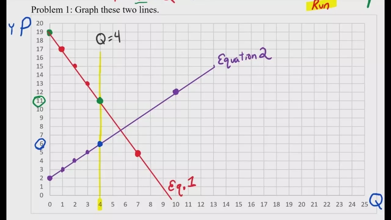















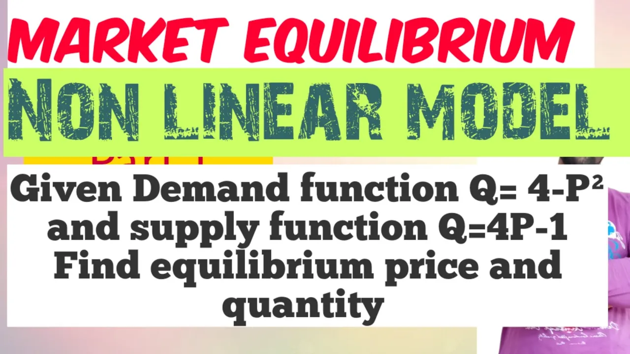




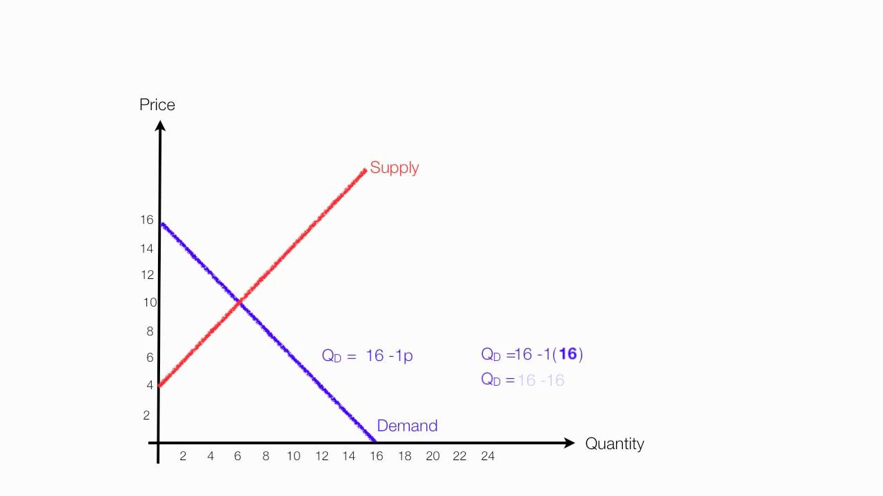


Market equilibrium occurs when quantity demanded equals quantity supplied; to find the equilibrium price and quantity mathematically, set the demand function equal to the supply function and solve for price, then substitute the equilibrium price back into either function to find the equilibrium quantity. For example, given QD = 60 - 3P and QS = -40 + 5P, setting 60 - 3P = -40 + 5P yields P = 12.5, and substituting P = 12.5 into either function gives Q = 22.5. Graphically, this is represented by plotting the inverse demand function P = 20 - (Q/3) and inverse supply function P = 8 + (Q/5), where their intersection point shows the equilibrium price and quantity.
Finding Equilibrium Price and Quantity from Demand & Supply Functions
Added:Basic algebraic skills, specifically solving systems of linear equations for unknown variables.
An understanding of the Law of Demand and the Law of Supply, including their inverse and direct relationships with price.
How to graph linear equations on a coordinate plane, noting that economics conventionally places Price (P) on the vertical axis and Quantity (Q) on the horizontal axis.
The conceptual definition of market equilibrium as the state where market supply and demand balance each other.
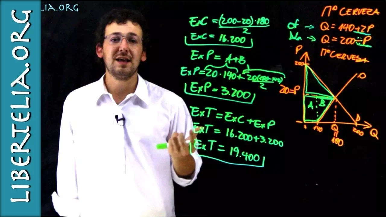
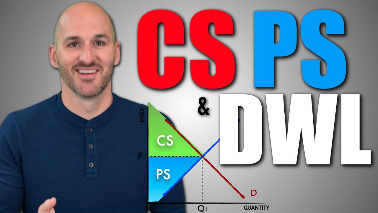
Calculating Consumer Surplus, Producer Surplus, and Deadweight Loss at the market equilibrium.
Analyzing market dynamics when demand or supply curves shift due to non-price determinants (e.g., changes in consumer income, production costs).
Evaluating the economic impact of government interventions such as taxes, subsidies, price ceilings, and price floors on equilibrium.
Applying mathematical derivatives to find equilibrium in non-linear supply and demand models.
Calculating the Price Elasticity of Demand and Supply at the specific equilibrium price and quantity.
102.9K views1.7Klikes8:42Original Release: 2020-07-15
hi this is hello in this video on mathematical economics series we will solve a numerical on how to find the equilibrium price in quantity when the demand and supply functions are given so the question is given demand function that is QD is equal to 60 minus 3p wire QD is quantity demanded and P is the price and supply function which is given as Q s is equal to minus 40 plus 5 P where P is the price and Q is the quantity supplied find equilibrium price and quantity so basically we have to find the market equilibrium now market equilibrium so we write here market equilibrium occurs market equilibrium is when quantity demanded is equal to quantity supplied now quantity demanded is 60 minus 3 P and quantity supplied is minus 40 plus Phi u P so solving this for P here we have this minus 3 P so we will transpose this Phi u P this will become minus Phi P so minus 3 P so I write here minus 3 P and transposing this will become minus Phi u P is equal to this is minus 40 minus 40 and transposing this 60 so this will become minus 60 so this is minus 3 and minus 5 is minus 8 this is minus 8 P is equal to so this minus 40 and minus 60 is minus hand rod now this cans this minus n minus L will get canceled out so 8 P is equal to hundred divided by sorry hundred and P is equal to hundred divided by 8 which is equal to 8 1 0 8 mm headphones are eight here it is 2 then it will become a twos are 16 so this is 16 2016 now here it is at fives are 40 so this will become 12.5 so our equilibrium price is 12.5 to find the equilibrium quantity we put the value of P is equal to 12.5 in either the demand function or in supply function so put P is equal to 12.5 in quantity demand so demand function we will put the value D are therefore Q is equal to 60 minus 3 this is 60 this is - this is 3 and the value of P is 12.5 so this will become 6 G - here three fives are fifteen point three to that 6 this is 7 and three ones are three so this is thirty seven point five when solving 60-37 point five is equal to twenty two point four you so our equilibrium quantity is twenty two point five now we have to grow up this also so let us in the axis this is the quantity axis and this is the price axis now to grow up this we have to find the inverse demand function and universe supply function to get the intercept here now our demand function is this to find the inverse demand function we will solve the given demand function Part B that is Q D is equal to 60 minus 3p or this will become 3 P is equal to and that is 60 minus Q so I will write Q in place of QD or P is equal to 60 divided by 3 minus Q divided by 3 so this is equal to P is equal to P is equal to or P is equal to that is three ones are 320 minus Q divided by 3 so for the demand function the intercept is here 20 and in the Arsenal it was here 60 so I will write it here this is 60 so our demand function is this similarly for inverse supply function we will find the inverse supply function data's solving this supply function parky oh sorry for P so this will become our Q s is equal to minus 40 plus Phi u P here I am solving for P also here so this will become this will become PI B is equal to 40 les Q or P is equal to 40 divided by 4 u plus Q do anyway for you are P is equal to 5 under five years are 40 plus Q divided by four you so here the intercept is 8 for supply function the intercept is here 8 and this is a lot demand function do-more and this is supply now equilibrium quantities that is this is the equilibrium quantity which here we are calculated that is 22 point for you and here this is the equilibrium price which we have calculated somewhere here that's 12 point 12 point 5 now given this data we can also find the producer surplus and consumer surplus so here the producer surplus is that area on the graph which is above the supply line and below the equilibrium price this is the supply curve and this is the equilibrium price so the area between the supply curve and the equilibrium price is the producers surplus so this is also producers surplus so this is producer surplus also the consumer surplus is the area which is below the demand curve and about the equilibrium price that is this portion represent this their consumer surplus this portion and this is the equilibrium point here so I hope you like this video if you want to find the videos on the mathematical economics you can search on my youtube channel that is econ maths on YouTube account maths so far more videos on mathematical economics please subscribe our YouTube channel economist also like comment and share if you like this video thank you
Up Next
12:31
Deadweight Loss Explained: Consumer & Producer Surplus
@JasonWelker
108K views•2016-09-07

5:07
Impact of Yuan in Indo-Russian Trade Amid Sanctions
@WION
261.9K views•2022-07-01

10:33
Behavioral Economics Explained: Rationality, Nudges, and Risk
@crashcourse
1.1M views•2016-03-12

113:18
The Age of Easy Money: Fed & Inflation | Full Documentary
@frontline
21.2M views•2023-03-15
Related Study Plans & Knowledge Roadmaps
Structured learning paths in Economics
economics
Sovereign Debt: Defaults, IMF & Restructuring
01Introduction to Sovereign Debt & Government Bonds
02Debt Sustainability & Credit Ratings
03Anatomy and History of Debt Crises
+ 2 more learning modules
12h5 modules
Explore Roadmap
economics
Market Design: Matching Theory & Gale-Shapley
01Introduction to Market Design and Price-Free Markets
02Two-Sided Matching & The Gale-Shapley Algorithm
03School Choice Systems and Mechanism Design
+ 2 more learning modules
10h5 modules
Explore Roadmap
economics
Impossible Trinity: Forex, Capital & Policy
01Introduction to Monetary Policy and Central Banking
02Exchange Rates and International Capital Flows
03The Mundell-Fleming Model
+ 2 more learning modules
8h5 modules
Explore Roadmap
economics
Healthcare Economics: Market Failures & Systems
01Introduction to Healthcare Markets and Market Failure
02Asymmetric Information and Adverse Selection
03Moral Hazard and Insurance Design
+ 2 more learning modules
12h5 modules
Explore Roadmap