Brownian Motion & Wiener Process Explained in Finance

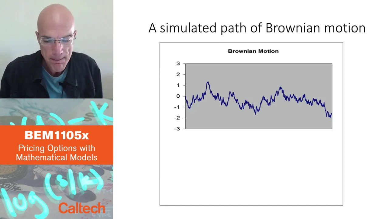
[00:00:00]all right so we're going to cover an introduction to a topic called brownie em motion which a lot of times in the financial um textbooks ends up being also called WEA processes but anyway just want to go over some definitions a process is a process is an event that evolves over time in attending intending to achieve a goal okay processes generally start at time equals Zer and end at time equals capital t it's typical notation of this during the time an event May at various points along the way have an effect on the eventual outcome of the event for example a baseball game baseball game happens over time let's say the innings are individual events that get added up to complete the process it is possible that the score from you know in a baseball game the previous scores get added to the score of the current inning to get the next score but it's doesn't for a process it doesn't have to look at the past so a process is basically a very vague concept it's just something that evolves over time and eventually is trying to achieve a goal a startastic process is a process which can be described by a change in some random variable over time which is either discrete or continuous so an example of a startastic process could be I don't know if you've ever seen questions in uh probability Theory where like you're trying to to predict today's weather and they say based on the last 3 days you put a weight on each of those and it'll tell you whether will rain or not rain today I know if you've ever had a question like that but basically the whether it rains or doesn't rain just keeps evolving over time and then you want to see um at a certain you could ask question like at a certain point in time what's the chance it would be raining when not raining so the process just counts on a random variable to figure out what it's turn Valu is so that's a pretty vague uh concept St testic process okay now in probability this is a famous cliche problem called a random walk a random walk is a statistic process that starts off with a score of zero and then at fixed points and times same interval between each of the fixed points and times discrete events uh there's a probability P that you will increase by your score will increase by one and a probability 1 - p u score will decrease by one and then this will happen this event will happen T times and then the walk is finished so one exam one question might be what is the expected value of your walk well you're starting off at zero so you're starting off at zero and then T times you're going to with probability P go up by one and probability 1 minus P you're going to go down by one so whatever that adds up to that's where you expect to be so for example if the probability was 50% chance you'd go up by one and 50% chance you'd go down by one each time an event occurs your expected gain would be zero right so you start off at zero you're expected to end at zero if there was a 75% chance you would go up by one and a 25% chance you'd go down by one then your expected gain would be a half right you'll either go up 75 or down by one so half the time you would go I'm sorry 75% chance you go up by one 75 * 1.75 yeah your gain would be a half so each time you're expected to increment by a half so where do you expect to be capital T units away T over two so if this if you did this 20 times you'd expect to be at 10 in a case like that okay and again random walks are discreet discret intervals like maybe it happens once every day or once every second but the amount of time is going to be the same okay again we're still on definitions a Markoff process is a so again a process is something that evolves over time a markof process is a process of a particular type of stasic process where only the present value and a very of a variable is relevant for predicting the future so an example of something that's not a Markoff process is if if you did have one of those examples where you look at the last three days tell can the weather for the last three days predicts the weather for tomorrow that's not a Markoff process because all you have to see is your current state today's weather to be able to predict tomorrow's weather you don't have to go back into the past to figure out um where you are currently so um so that's a Markoff process and then uh the inry of the variable and the way that the present value merge of the past are irrelevant okay now a Martin Gale process hopefully we near the end of uh going over definitions but a Martingale process um Mar out process is a stasic process where at any point in time T the expected value of the final the the expected final value equals whatever the current value is so let's say for example you had a random walk and the random walk after let's say it's supposed to run for 20 time intervals and after 14 time intervals the current value is four then the final value is expected to also be four so what this is basically saying is at any point in time you could randomly pick a point in time and say from that point until the end I expect to see no change so what would that actually mean about the probability of what's come the events that are coming up the upcoming events have an expected gain of zero they're not expected to up not expected to go down so for example if you had a mod Gale process like a random walk you start at zero and you start going up or down up and down you eventually get to minus 4 and then you said what do I expect it to be when this thing eventually ends if it hit minus four at some intermediate point if you said well I expect it to be minus 4 I don't expect to be a positive or negative change from this point on that would be a morning Gale process so does that make sense that that a process that basically says this notation is basically saying at a point T along the way the current value is X so where do you expect it to be when it finishes well I expect it to be X CU I don't think anything that's going to happen in the F what's going to happen in the future has no expected gain or loss and all Mar Gales by Nature are Marian so again Marian means you don't need to see the past of how it got to X all you need to know is it's currently at X and it's expected to stay at that okay so this is something I just did in matlb this is a a tool uh we can use to kind of generate or simulate things we're doing so I basically coded up in mat lab I started with a value of zero and then at each time interval and I did 100 time intervals but I basically said at each time interval I'm going to e you know I I simulated a coin being tossed that had a 50% chance of being heads and a 50% chance of being Tails if the heads came out I incremented my score by one and if a tailes came out I decremented my score by one and then just let it run a 100 times and then each time I let it run I changed the color of the random walk so for example the blue random walk went like this like there two blue oh must yeah it must have done two blue Rand walk so then it went like along this path and eventually ended up down here and then for example this yellow random walk went like this now if at any point in time so a a random walk is by nature of Martingale at any point in time let's say say for example I started at one and this yellow one went along here so here it had a nice streak of head head head and then eventually went Tail's head but let's say at this point at this point in time it looks like I'm at about 8 or n my score right now is at eight or nine if you were asked where do you expect to be when we hit time equals 100 right now at time equals 60 after 60 coin flips I was at Plus 8 right about plus yeah it looks like about plus eight where would you expect me to be at time equal 100 if I if the only piece of information I'm telling you is at 60 I was at Plus 8 where would you expect i' be at 100 you'd expect me to stay at Plus 8 I may go up I may go down but the chance I'll go up equals the chance I'll go down I should expect to stay at8 and then what you might see in uh the textbook it says that it uses this term of filtration so it basically says the definition of a modding Gale is a process who based on a current value and a current filtration you can expect the future value to be exactly the same as the current value and what we basically mean by a filtration is this suppose I told you suppose I let this run to time equals 60 and at time equals 60 the value is 8 but suppose I I also told you at time equal 40 the value was three and at time equal 20 the value was four suppose I gave you three pieces of information what the value was at time 20 what the value was at time 40 and what the value was at time 60 with all three of those in pieces of information if I said what do you expect it to be at 100 what thinking would you do if it's a Maring the value of 20 and the value of 40 really don't matter it's the most recent piece of news just to basically you're filtering out the not not needed pieces of news and you're just taking the most recent one and saying well okay if you're telling me at time 20 the value was four at time 40 the value was three and at time 60 the value was 8 and with those three pieces of information you're asking me to predict what will its value be 100 I'm going to ignore 20 and 40 I'm just going to take the most recent piece of news and say since this is a marale its expected value at any going into any future is it it is expected to not change so I would just say Okay then if if at 60 the value was eight I expect it to finish at eight that's a mar okay so this is just a a set of what they call sample Paths of a random random walk so a random walk is a probabilistic thing it has no you know it's a it's a random process each time you alter the score by whatever the random event was and you just keep a running total so each one of these lines is called a sample ad of a random walk so you'll see that a lot in the textbooks they'll go over sample pths and okay so now a formal definition of a Browning motion and what I'm going to do in a couple slides is basically take a a random walk and convert it into a brownie motion but the formal definition of a Browning motion is a stasic process so all these things we're defining tonight at processes they happen over time a startastic process and it's popularly use the letter w w you would think you would use B but some books use B for Browning and some use W for uh wiener um but it's a process that happens over time from zero off to Infinity is a standard Browning motion if number one it starts off at zero so just like the random walk we could have made it start anywhere but we decided to start it at zero it has continuous sample paths so the random walk doesn't have continuous sample pths it it has discrete points where the value jumps and actually in the in that mat mat lab uh diagram I drew was actually drawing an angle to get from one point to the other it actually should have just put dots at each of the points and let your mind connect the dots but it actually drew a line between them but this is a has continuous sample paths and it's it has independently normally distributed increments so this the random War had a uniformly distributed increment they either had a 50% chance of going up or a 50% chance of going down this one as we go from one value to the next one the way the what we use to get to the next one is we run a Rand a I'm sorry a normally distributed variable and see what its result is and then add that to the current score so the random walk is again we start off with a current score of zero we then have a random event occur that has a 50% chance of going up and a 50% chance of going down and take that outcome and add it to our current score and we just kept doing that until we got to the end of time in this case we're going to take our current score which starts over at zero run a normally distributed random variable add that result to our current score and that gives us our next score and we will do that until the until we hit capital T now unlike the random walk where we go where the time between each random event is discreetly scheduled these happen instantaneously so when one happens the next one happens instantaneously after that and if you remember from the central limit theorem adding together a bunch of uh variables with pretty much any distribution will add together and BEC a normally distributed uh process okay so this ends up being kind of a formal definition and shortly we'll talk about how to build one from a random wall but what's going to happen a lot with our with our textbooks and just in this field a Brownie and motion which we said was a process and it was Brownie and motion was named after a uh kind of like a botanist like a who's people who study plants what do they call Bist I think you're right botanist okay so he was a BST from maybe 150 200 years ago and he was kind of studying like when pollen Falls in a lake how how long does it take to move around the lake and it was kind of like where is its current location well it's it's its current location plus a normally distributed variable will give you its next location I was kind of studying that and so that's why a lot of the older textbooks refer to this as a brownie motion this type of process and then there was a mathematician if it was a mathematician but a a uh famous person by the name of weiner I think uh I think I was reading he like finished College when he was 11 and finished a PhD at Harvard when it was like 17 but I forget if it was in math but he ended up making big contributions to mathematics and so this is sometimes referred to as a weener process so branding motion and weener process you'll see in the literature end up for the most part meaning the same thing but a ween process is basically a uh a process characterized by three facts like the Browning motion it starts over at zero in this case that has almost continuous simple uh sample paths browny motion said it had simple um sample pads this one allows for us to have two points in time time T and Time s the gap between those two could be normally distributed with a mean of zero and a variance of T minus s so this kind of opens the door between Bridging the grounding motion and kind of that random walk and saying the two can be somewhat similar if the gaps between the event got really really small and many many gaps so as as the sides of the gaps go to zero a random walk starts to become a browning motion and a weener process could be somewhere between the two kind of opens the door that it could be somewhere between these two but as far as our textbook is concerned um and kind of this field is concerned grounding motions and weing processes can be um can be considered the same thing okay and that's why actually a lot of a lot of the definitions said a brownie motion is a process WT and the W ends up being come coming from the name wiener so you might see in the textbook they might describe a brown em motion and use the word I use the letter W to symbolize and then if you want we could have many dimensional Browning motions we could have a vector of uh brownie motions and it's an end dimensional brownie motion if each of the W's which is the brownie motion process um is a standard brownie motion and are all independent of each other so that's a definition will just pop up later on okay so now what we're going to just try to do is convert the random walk into a Browning motion okay so um so if we took a random walk and instead of doing like we did originally where I said uh every time interval let's say you know there's a there's a a gap of time capital T and then they broken up into little small T time intervals discreete time intervals instead of saying that the next event the thing we're going to add to our current score instead of that being a uniformly distributed variable 50% chance plus one 50% chance minus one I'm going to say it's a randomly I'm sorry it's going to be a normally distributed next event with a mean of zero okay now suppose we decided so first change we're making to the random walk is we're saying the thing we're adding to our current score is normally distributed not uniformly distributed the second thing I want to do is to take the interval each of the intervals Little T that we add or subtract to our score I want to divide that up into n equal parts some number n now obviously we know from continuous mathematics we're going to eventually let N Go off to infinity and see what happens that's the way calculus works okay so each of the increments if we take what used to be our only increment which happens at time T and now divide that up into n intervals each of our increments will add this much to our would have expected to be add this much to our uh score and the total increment Si would equal the sum of all of these uh residual increments the expected value of all of them added up since this is a Martingale would be zero the expected value of each of the increments would be zero actually I probably should have wrote I should have wrote these the other way around this is the individual ones adding up and this is the sum of all of these would be expected to be equal to zero the expected value for r s since r i is equal to we're letting this be the root of t n for it to be a normal uh normally distributed variable r s is expected to be T over so the expected value for the increment would be zero but the expected value for the variable squared would be T over okay and then we have the expected Val so now we're going to start to calculate we're going to start heading in the direction of calculating the variance so this of of course this is a a weener process or a uh grounding motion it's a Martingale process at any point in time the expected increase would be zero but we want to calculate we want to start heading towards calculating the variance so the Val of s s because it's the value of s s minus the expected value of s that whole thing squared we use that to calculate the variance the value of s² would be equal to all of the increments the value of s squ up to some point in time I would be all of the increments from 1 to I times itself and then take the expected value of that so this is going to end up having a lot of terms this would be linear but there would be a lot of terms it would be R1 * R1 + R1 * R2 + R1 * R3 we go through that whole row then it would be R2 * R R1 then R2 * R2 R2 * R3 and so on if we said that each of these individual bits now that now that we're taking the random walk and slicing them up into n Parts if we said each of those were independent of each other then there would be no correlation between anytime I and J were not equal to each other there'd be no Cor coration so the expected value of any two random variables that have the same expected uh that both have an expected value of zero multiplied together would also be zero so since I and J are not any combination of I and J as long as it's not the same one were uncorrelated the expected value of this tus would be zero so a lot of the terms in this we're trying to calculate s s you know the expected value of s squ a lot of these terms would get end up getting zeroed at the only ones that would survive would be the expected value of s s would end up being R1 this is kind of a PowerPoint notation these should be lined up the one and the two on top of each other but R R1 squar plus and we go all the way down to r i s so it would be I terms each having a value of T Over N so the expected value of s² would end up being for example if we went as far as up all the way up to n would end up being n * T Over N which ends up being T so the value of the expected value of S2 would be T the way we took the random walk and chopped it up into little pieces and chopped it up into n Pieces it's expect the expected value of s s would be T the expected value of s the expected value of s with the squared on the outside would end up being zero right because the expected value it's a monate so it's expected value would be zero so the variance would end up being T minus 0 which ends up being T so the the variance of this process and all we've done so far is we've taken a random walk and instead of it just being a fixed a set of fixed intervals with one result we took those fixed intervals and cut them up into individual equally sized pieces and had each of them add a uniform uh a Rand a normally distributed variable to those for each of the end pieces and we end up figuring out what its variance would be so we know it's expected value because it's am monil is zero its variance would end up being T so now what we'd like to do I think the next step should be you have to let N Go to Infinity so as we let N Go to Infinity if we take a random walk and take each of the time intervals and cut them up into n equal slices and then let N Go to Infinity this is now a um this is now going to be a random walk where every event happens immediately after the previous one and we keep taking these really incredibly small increments or decrements which are normally distributed and add that to our current score the expected value at the end of the process as n goes off to Infinity we end up with a we're going to say now a different function and that different function now becomes a brown in motion so we basically used instantaneous mathematics to go from a discrete scenario to an to a continuous scenario and this function which we'll Now call X of t is called the Browning motion that corresponds to the random walk if we let it slice up and let N Go to Infinity its expected value once again it is a um it's a Maring Gale so it's expected value of zero a normally distributed uh variable is has a bell curve to it so we're always adding something that has an expected value of zero to our current score we expect our curent score to stay the same and the expected value of x s ends up like we said before being which then also contributes to the variance of this okay so then uh note that a brown emotion is Marian meaning all you have to know to know what its next value is is its current value and what we're adding or subtracting from it we don't need to know the history of how it got there that makes it morovian it ends up being finite now that we let N Go to Infinity this became a continuous variable it is a marting because it's expected value from wherever it currently is it is expected to not change and it is normally distributed with a mean of zero and a variance of T and okay so where are we really going with this so this is kind of the last thing we'll talk about today where is this really going what's the point of this suppose we had a differential equation of this form we're saying DX the rate that some variable X changes is equal to a DT plus b * the derivative of what we're now saying is a Brownian motion or a Weena process okay where A and B are constants okay now the DX equal a DT part this part let's say this let's say this was not here Pretend This part's not here so it's just DX = a DT what would that integrate to if you were solving that differential equation what would that integrate into that would turn into x = a t plus some constant so some initial value of x and then we're going to add an A and A T and T ends up in in this case end up being time so this is basically saying like we'll start with some initial value and then depending on time we'll just keep whatever the time is We'll add that many A's to the score so what are we effectively doing here we're taking some initial value and then making it go assuming a is uh positive in finance it'll be positive but in any other thing it could be posit POS or negative but we'll say this is positive we're going to take some initial score and then at times going to cause the value to go up this is going to be kind of like the current stock price and then this would be maybe interest an interest rate on it or something that something that goes up over time so we're going to say like the current price of something is equal to its initial Price Plus as time goes on its value somehow inflates it inflates by a if we we wanted it to be a rate I guess we'd have to say whatever x0 is multiply that by like R this would end up a would end up being rx0 so that would be like for example if we wanted to say a stock price is let's say a stock price is currently $100 and we want to model where is it going to go in the future and suppose we said it's going to just be its current value plus interest so it's not really a stock it's kind of like putting money in the Bank it would be the current price is equal to the initial Price Plus the initial P Price times some rate times time so let's say it was initially $100 and the rate was 2% you take 2% time 100 which is two every time unit maybe the time units could be years every year you get an extra $2 so be like $100 time plus two plus two plus two something along those lines so we can start using an equation something like this to model the value of something that grows over time yeah so um XO that's the that's what it's um initial is and then X is the current yeah X would be the current so this is some initial uh this is so this is basically a modeling equation so this is like what we initially started with and then time causes us to add some value to it actually a could be negative which which could make value go down down which could be in the case of you know present value future value if it was going down but what we're going to end up doing is we're going to say we're going to model the price of something by saying it's whatever it initially started as we're going to assume in the case of things going up with respect to interest this is this part of the equation is going to be the interest part the part where we say okay the more time we have the more it goes up over time so we'd have to let a or whatever we put in front of the T something that models the interest based on whatever the carent price is now that would model this equation alone without this piece would model um an amount of money that was growing at a very fixed rate with absolutely no volatility there's no it's just like putting money in the bank and getting guaranteed interest what if we bought stock which may go up may go down but has an expected increase rate like when you buy St you expect it to go up with the interest rate but it might go much higher it might go much lower but you have an your expected value is it should at least compete with interest if you're a risk neutral minded person it's got to at least compete with interest so when we go to model it when we say the rate of change of the stock it should be equal to two it should have two components to it it should have and now this isn't this is one thing I said before I say this this is not the perfect model for a stock but this is the most most commonly used one so we're saying the price changes it has two components to it number one what we have something that models the interest rate something that grows with time a second component is just some variable part that could go up could go down and it's going to go up using it's going to be a wiener process which starts at zero and then make might go up might go down and then we're going to multiply it by a magnitude and add that number to the constant rate going up to take a guess at where it would be at some point in the future so this is the model we're going to be using so the two components are the first component is exact interest and the second component is a wiena process which is just moving up and down as time goes on and we're multiplying that by a fact B what what would the factor B be in the real world so this is the this is the fixed component and this is the variable that we might win we might lose but we're going to map along the idea of of an interest line and then maybe go up or down along that line on a on a based on a Weena process why would we have a magnitude of that one stock might vary a little bit and one St might vary a lot and that magnitude would end up just being a bigger number for a highly variable stock so a stock like Google might have a big number for B and a stock that doesn't change much like a soda company like Coca-Cola might not change much that might have a very low be the Weena process Weena process is always the same thing starts at zero and then just keeps adding instantaneous increments of a normally distributed variable they all have the same magnitude so if we want to make a stock seem more volatile than another we just make we make B larger and if the interest rates go up we make a larger so the a constant here controls the interest rate component of our predicting the stock and the wiener process multiplied by some magnitude gives a Randomness to the stock and the B makes the randomness either bigger or smaller and so what we're going to do is take those two concepts add these two components together and then say this is what we're going to use to model the behavior of a stock so the interest rate part will come from whatever the current interest rates are we assume that whatever today's interest rate is is going to be the same a year from now if we're trying to figure out what the price is going to be a year from now and we're going to make the assumption that the volatility of a stock from the past will match the volatility of the stock from the future which is not always true but that's the only thing we can do say the past volatility we guess that's going to be the same for the future so what we can now do is we could using something like matlb is we can program in all these numbers based on the current interest rate and the past volatility of a stock and then say here's what the stock might do and let it run do like I did with those uh random walks let a bunch of sample pths run it's going to be random and then if we wanted to so like I say maybe I'll do uh next class I'll do a a brownie motion version of it but when we did this let's say instead of these being a bunch of random walks suppose these were a bunch of uh Browning motions if these were a bunch I'm sorry if these were yeah if these were a bunch of browny motions rather than a random walk if we added an interest rate we'd be taking all of these and slightly tilting them up so they' be going like in this direction not not out like a Martingale but they' going up on an angle and then we'd say okay the possible results based on the volatility of the stock we would have you know a wide range less volatility they'd be closer to the middle but still angling up at the interest rate and then if we wanted to say what is the price of a stock option on this stock with let's say a call of this number that means from this number and up we get profits from this number and down we don't get anything so we would take we could run this experiment thousands of times take all of the numbers above the strike price take an average of them and say that's what we think we're going to collect in the future and then subtract interest or discount by interest back to today and that's what we think the stock option would be worth if we use that model the equation we had before to model the stock correctly then run the experiment thousands of times take a weighted average we could guess what the a stock option would be worth today so this was kind of the the groundwork of uh the method that was used by black and SCH black sches and Martin I think came up with using this model and that equation by taking the saying the price of the stock will be take its current price add add constant interest to it and then add a we a process with a magnitude of volatility based on the past to predict the future and then take um calculate an expected value for the co price so that's what we'll talk about next class uh if you want to read up ahead it's the black sh black there's two or three people black sh s c and and Morton sometimes that name shows up and they won the Nobel Prize for this calculation how how to calculate the price of all options won a Nobel Prize