




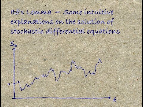





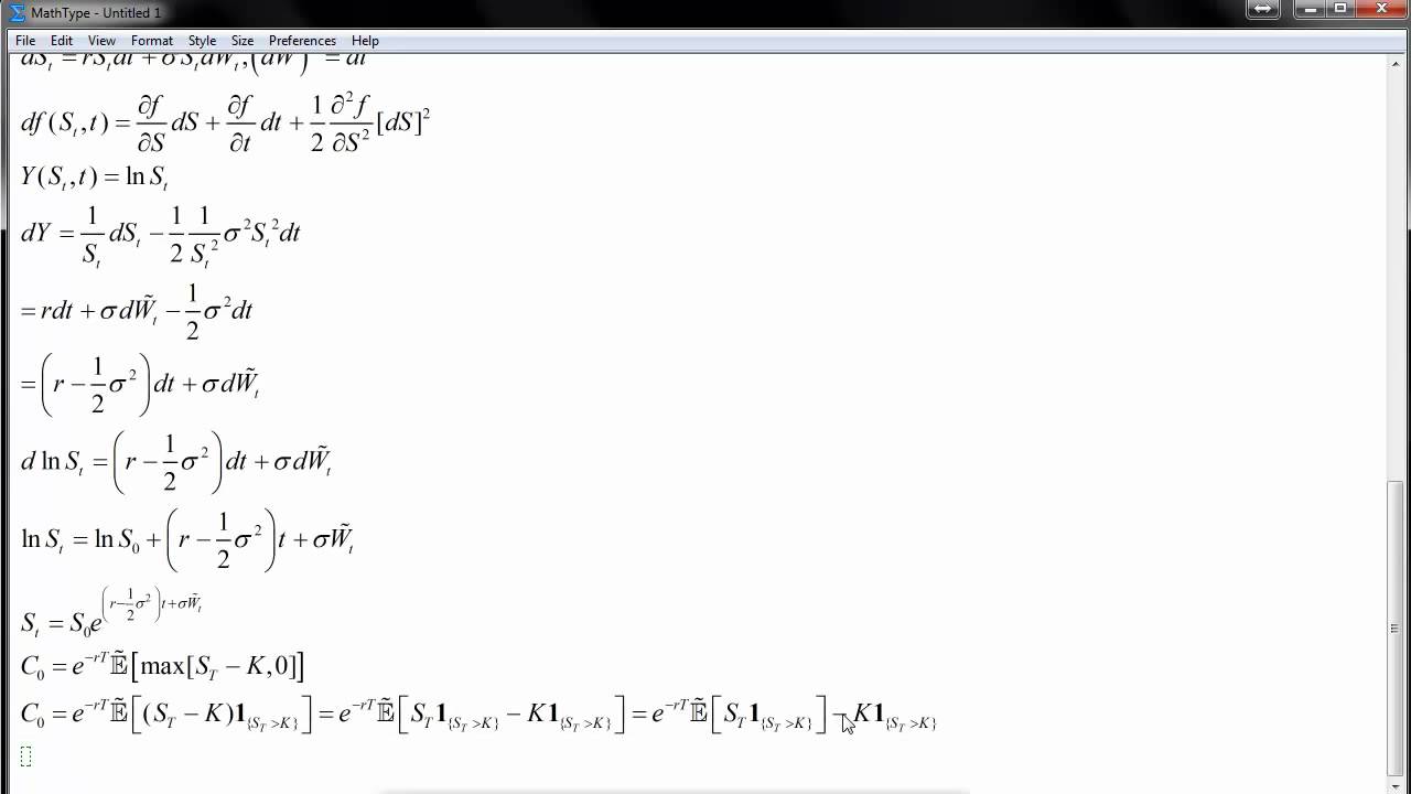





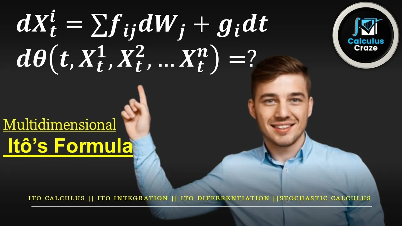
Ito's Lemma is a fundamental theorem in stochastic calculus that allows us to find the differential of a function of an Ito process. Specifically, if a process X follows the stochastic differential equation dX = a(t,X)dt + b(t,X)dW, then for any twice-differentiable function g(X,t), the differential of g is given by dg = [∂g/∂x * a + ∂g/∂t + (1/2) * ∂²g/∂x² * b²]dt + [∂g/∂x * b]dW. This lemma is essential for modeling financial derivatives, as it enables us to derive the dynamics of complex financial instruments (like forward contracts or call options) based on simpler underlying processes (like stock prices), by computing the appropriate partial derivatives and applying the formula.
Ito's Lemma in Financial Mathematics: Derivation & Applications
Added:Multivariable calculus and Taylor series expansions, specifically understanding second-order partial derivatives.
Foundational probability theory and the definition of a Wiener process (standard Brownian motion), including its properties of independent, normally distributed increments.
An introductory understanding of ordinary differential equations (ODEs) and the transition to stochastic differential equations (SDEs).
Basic financial concepts, specifically the mechanics of asset prices, risk-free rates, and derivative instruments like forward contracts.
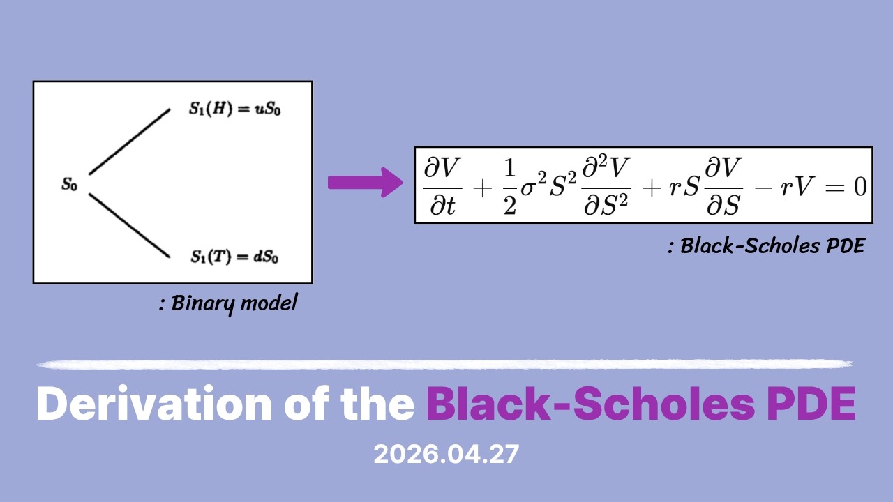
Derivation of the Black-Scholes-Merton partial differential equation (PDE) for option pricing using Ito's lemma.
Girsanov's Theorem and the concept of change of measure (transitioning to a risk-neutral probability world).
Numerical methods for stochastic differential equations, such as the Euler-Maruyama simulation scheme for path generation.
Applying multi-dimensional Ito's lemma to model correlated assets, interest rate frameworks (e.g., Vasicek or Hull-White models), and credit risk.
141.6K views1.4Klikes37:39Original Release: 2011-11-15
Okay. So, tonight I want to talk about Ido's lema, famous famous lema about uh brownie motions and using a function that is described by a brownie in motion to create another uh statement about that function. So, I'll be going over um eo eto processes and and also geometric browning motion to start off with. Okay.
So by definition a geometric brownie motion is uh basically this is one where uh the we're not going instantly. We're not we're not taking gap time instantly but the change in a variable and we'll use s because eventually this will become a stock price. The change in the stock price divided by the stock price ends up being we'll use this Greek letter multiply that by the change in time. So this will map to being our interest rate.
So we'll take that amount and then we'll take sigma which will be which is going to eventually map to our standard deviation multiplied by an epsilon which is a standard normal. So that would be a a normally distributed random variable with a mean of zero and a standard deviation of one. And then multiplying that by the square root of the amount of time we let go through. Then multiplying both sides by s we get this formula. So it's really two different ways of saying the same formula. So again the delta s is the change in the stock price or whatever s is.
Mu ends up being the expected rate of return. So the more time you give it is this is how much it goes up by.
And again this is a discrete case. So this is not a continuous case. Um sigma is the volatility of the stock which will map to a standard deviation.
And then the sigma time the epsilon * square roo<unk> of delta t is the stochastic component and its variance is this part uh the t the this component squared without the normal part taken out. So this ends up being the variance because that's the standard deviation squared. The stocharastic component of it is the part that we can't use standard calculus on.
We can't use the remon sum model for integrating.
Okay.
So we needed a type of calculus for this type of uh for this type of um mathematics. And then a famous mathematician, a Japanese mathematician by the name of Ido um who passed away a few years ago, but he came up with a uh lema about processes like this. So we'll talk about what an e process is and then if you have an e process, we'll apply this lema to it to give us another process and that other process will provide us some uh interesting information. So anito process can be generalized as a wiener process in which the parameters a and b um are functions.
So they they don't necessarily have to be constants but we'll be doing examples where they're constants and somewhere they'll be functions.
So a and b can be a function.
And then we're going to model um a will end up representing some type of rate of growth and b will end up representing a magnitude that we're going to multiply the wiener process from. So you may have seen this as a z in your other textbook.
The bz here.
Okay. So some textbooks you'll see this as a b for browning motion. Sometimes you'll see it as a W and sometimes you'll see it as a Z. I don't know where the Z comes from, but um okay, and this is where the W component is an M dimensional standard brownie motion and the A and the B end up being N dimensional. So we this actually this formula applies for where we could have many stocks. It doesn't have to just be one stock. We could have a collection of independent stocks and this whole formula would apply to it.
Okay, so basically we're saying the current price of a stock at any point in time is equal to what it started off at time zero. We're going to integrate from zero up to a point t. Integrate add up all the uh interest we gain. So this will end up being um just the pure gain of interest. And then this will be the randomness of the stock. This will be some magnitude times a wiener process.
And then we just add that up over time.
Add the whole thing together and that will give us a model for what the stock price will be at any particular point t in time.
Okay.
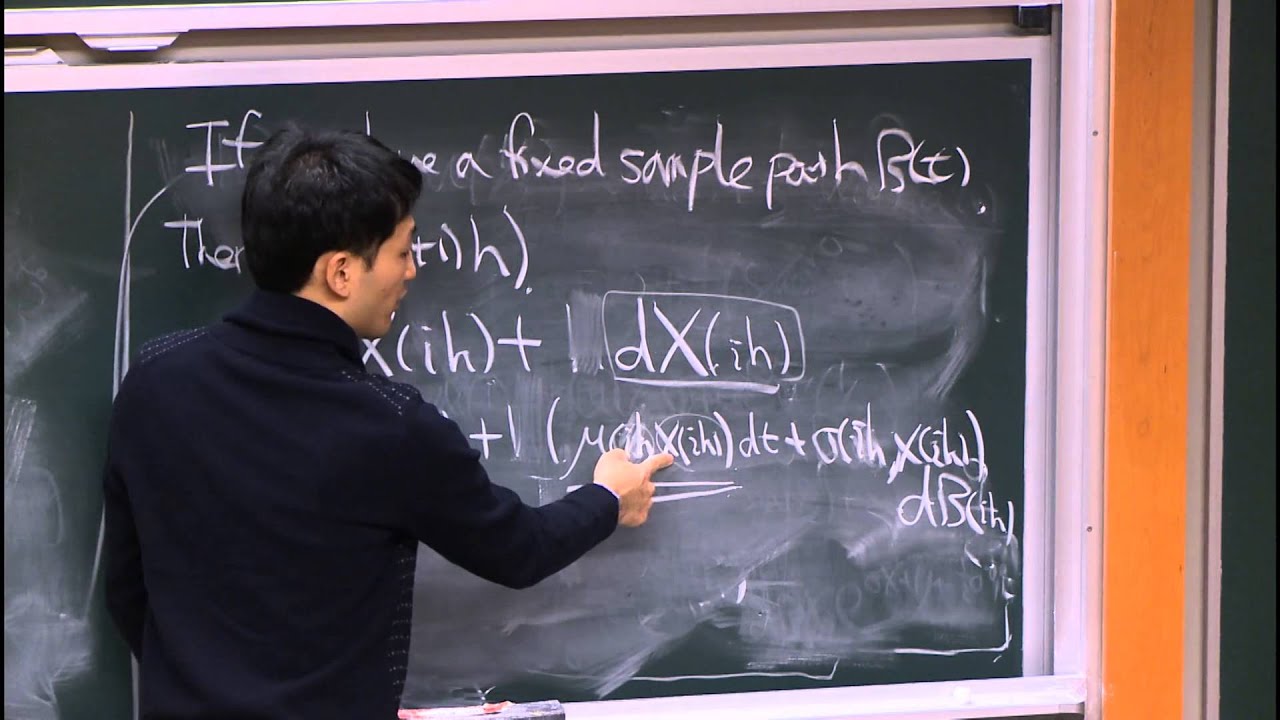
So then just continuing on another way to write that integral we had before is write it as a differential equation. So basically this equation is the derivative of the previous formula. So instead of it being xt, we take the derivative of it. And then the integral part, we take away the integral sign and we just get a of tdt b of t d w.
So this ends up being an n- dimensional stotastic differential equation which has this form. So we end up we like I said before we could use this in the simple cases this could just be a constant and this could be a constant otherwise the variable a which is the component of growth could be a function of the stock price and time and it could again it could just be a constant if we wanted to this can also over time and over the price uh change in the stock stock price could change too. So this is the more general case and we now have a differential equation and we also have an initial condition that the stock price originally started at some number. So in a concrete example we might say you know IBM stock is currently at 100. How would you model where it could go into the future?
So this ends up being a differential equation but because there is a stochastic component of it we can't use normal differential equations to solve this.
If we then were to integrate this equation, we'd end up back with this differential equation, the one that we had before. Actually, probably should have put a subscript of zero here.
Okay, so now this this component since this is a function of just the stock price and time, we could use standard calculus to solve this component. This one we couldn't because this is being multiplied by a wiener process which we can't do standard integration on.
Otherwise we'd be able to just solve this differential equation using standard methods of solving differential equations.
Okay. So Eido's lema and we're not going to go over the proof of this. Um Ido's lema basically says this. It's this is a very powerful um statement and when we go over some examples next well yeah at the end of this these slides and also next um we'll see an example of this but it's basically saying this suppose you have something that follows an eo process meaning its rate of change equals some component times time so it's growing at a rate and then also has a variable part to it. A a part with a I'm using Z. So you can tell I copied this from two different textbooks. This Z is the same as the W from the last slide.
So um so and then this is a compon this is a magnitude being multiplied on top of the wiener process. Okay, this is where DZ is a wiener process and A and B are functions of X and T.
If this is true, let's say you have some process that is modeled this way, then you if you have another function, any function, you could actually make up any function, any function g, which is of the variables x and t. So this would be like our stock price and this would be time. This statement in red is always true.
The rate at which the g function changes is equal to the first derivative of g with respect to x * a plus the first derivative of g with respect to t plus 12 the second derivative of g with respect to x * b ^ 2. You multiply this component. This whole thing gets multiplied by dt and then also plus the first derivative of this function g that you've made up with respect to x * b gets multiplied by the same wiener process.
So what this is saying is if you could come up with any process that's modeled this way, if somewhere out in the real world there's a process that's modeled this way and we could kind of argue that stock can be modeled this way. So yeah, let me just take a second to talk about this.
Stock can be modeled in such a way that it's variable. It has a randomness. It could go up or down. Some stocks are more volatile than others, have a history of going up and down at a much higher rate than those. And that's why we use this here to multiply how much variability there is to it. In addition to that, in investors expect on average risk neutral-minded investors expect to make money at least at the rate of interest. Otherwise, they just put the money in the bank and gain interest. Why would they buy stock? So, there should be a component that as you multiply it against time, there's expected growth.
So we could make the argument that we can model stock with a this stotastic differential equation.
Now some people might argue this doesn't perfectly m model stock. So I just wanted to point this out. This component could since we don't have any control over it. It's just a random process.
This could get so big that it's bigger than this part and then the whole the price of the stock could theoretically go negative here. But in the real stock market, as the price of stock gets near zero, the company closes and it never goes negative. But in this model, we could actually go negative.
So it's not a perfect model for stock, but yet we can use this to model stock.
Now the question is if this is the model for a piece of stock, you could turn around and say, well, I have a new function G, which is basically 2 * X.
That's a really easy example. Gals 2 * X.
Then the rate at which g changes ends up being this formula. So we we have the freedom now to make up any function g which takes as input x and t. This statement about the function g we've made up will always be true. And if you think about it this is another process right? What is an ed process? The rate of change equals something time dt plus something time dz. And that's what this forms into.
So we could take any eido process make up any function we want any function g we want and this statement will be true. So the g function will also be an eo process and it's just a matter of calculating these first and second order derivatives and plugging in the formula. So this unfortunately ends up being a formula you have to memorize because it's not easy to just uh off the top of your head remember it. It's not intuitive. So you know any test question hopefully the teacher puts that on the test. So it's just a matter of finding out what the function is and then taking those components and putting the formula together.
So an eo eido with drift and variance basically is saying this. Um so oh yeah like I said last time the g function which is any function we can make up but uses x as input. Um that will also be a eo process. It has what we're now going to call a drift rate. So drift rate is basically as time goes on it's angling upward on average.
So the first component the big component in the middle ends up being the drift.
So let me just explain what I mean by that. So the eo process has two components to it. Uh the two components are what we're calling the a part or this component is basically making our process drift on an angle upward. I'm assuming this is positive. I guess we could have negative interest if we want or in a non-financial sense this could be a negative number but in the financial world this will always be positive and this will cause our pro process to drift upward. And in the risk neutral-minded sense, it would drift upward at the rate of interest.
So the new component, the drift part, this part is the drift part and this could be the random part or the stotastic part, whatever you want to call it. This ends up being in based on Eido's lema. This ends up being the drift component. And then this component ends up being the new stochastic component.
And I'll go over somewhat of a concrete example um shortly. But what I'm basically saying here is this is the drift part. The drift rate this whole component gets multiplied by dt and the variance component. This was the square root of this ended up being the term in front of the eos I'm sorry the in front of the uh wina process. And then if you just square both sides you get the variance of it.
Uh and I'm just saying no we're not going to derive Leo's lema here. Uh that would go that would be covered in a start testing calculus class the derivation of it.
Okay. So um let's apply this to something a little bit more concrete.
So we're basically saying we now have this interesting lema which basically says if you give me an edo process I can go and make up any formula that uses that eo process as input and the new thing that I've made up follows the eido's lema formula.
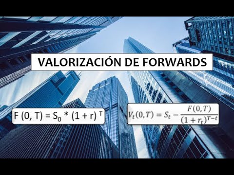
So let's say our inputting process is a stock price and the new thing is a forward price on that stock. So if you remember a forward price uh if you if you had a stock and you wanted to know what the forward price is, the formula would go like this. The forward price is equal to the stock price times interest. We would add interest to the price. So for example, if a stock price is currently $100 and the interest rate is 5% and time equals 1 year, what should those two people agree that the forward price should be one year from today? That would be $105, right? We remember this from forward. So the forward price would be 105 as of today. Now, as time goes on, the forward price keeps changing, right?
So, we want to come up with a model for the forward price.
We have a model for the stock price.
We're using what we said before, the the formula where the stock goes up at a normal interest rate and plus has variability to it. We'd like to come up with a model for the forward price. So, we are interested in a forward price as time passes. Okay? Okay, so we'll let F be the forward price, S be the stock price, and at any point in time t before the year ends or before the term ends, this formula would be true. The forward price should be whatever the current stock price is.
And then also we would want to tack on interest from now little t until the end of the term of the the uh contract. So this formula will tell you the current value of the forward. So as the stock price is jumping up and down, the forward price is moving differently, right? In fact, if the stock price was angling upward with the interest rate, the forward price would stay completely constant. If the stock price starts shooting up, the forward price will shoot up, but at a with a different process, too. So, does that and and like I say, maybe um next week I'll go over an example of these two where we can graph the two together.
But what I'm I just want you to try to imagine is as the stock price is moving around, the forward price is also moving around with it but differently.
And this function, so this would be like on our on our ETS's lema, this would be our G function. We get to make up any function that takes an eido process as input and eido's lema becomes true about it.
So if we wanted to take this as our G then based on Ido's lema this statement should be true.
Everywhere you see a G here, change them to F for forward. Like I said, G is just any function we can make up that uses X as input. Now S, if you change the G's to Fs and the X's to S's on that last formula, this statement about our forward price is true. This is the thing EDO proof. This will be true in all cases.
So that's our f formula.
So now we just go and calculate the what do we need? We needed two first order derivatives and a second order derivative. We need the the derivative of f with respect to x * a. We need the derivative of f with respect to t. And then we need the second derivative with respect to s. f second derivative with respect to x. So we'll calculate those out separately.
So based on this formula at the bottom of the screen, we calculate these three derivatives.
So our first derivative of the forward price with respect to s ends up being this based on the formula from the previous page. the second derivative of the forward price with respect to S with respect to S. There's no stop term here. So derivative of a constant is zero.
And a lot of the easier examples in the textbook, the second derivative comes out zero. They get a little much bit of a pain when you have when this thing is not zero. And then the derivative of our forward price with respect to time ends up being this. So if we take these three terms and plug them into the EOS lima formula, we should get this.
So I actually rewrote Eido's lema and then plugged in our this is the Eido's lema in general. Um but I use F instead of G.
I probably should have made those G's just to say we're taking Eido's formula and then plugging it into our special case. But anyway, so what I'm saying is the the calculation we came up with for the forward price.
We said the forward price equals the stock price with the interest, you know, the exponent being BT minus little tacking on that much interest. We came up with a new process. According to Edido's lema, this statement is true.
And hopefully this will help us somehow.
But we're basically saying the rate at which the forward price changes is equal to the first derivative of the forward price with respect to the stock price times mu which is the rate it increases times the stock price plus this is the first derivative of the forward with respect to time. That was the green component from the last slide.
Then times 12 the second derivative of the forward price with respect to the stock price with which ended up being zero times sigma s 2 which all this will get all zeroed out plus this is the uh stotastic component where we take the derivative of the forward with respect to the stock price which ended up being this part multiplying that by sigma * s times the wina process So this whole thing is now a new wina pro uh this whole thing is now a new um eo process.
It drifts upward at this rate this times dt and this component actually this component ends up being the standard deviation of the forward that maps to this stock price.
And we can this little more simple. Okay, we can substitute f for everywhere we see s * e to the r tus d because we said those equal each other. So we can rewrite the previous equation. If we collapse everything together, we can rewrite the equation on the bottom in the different colors can actually be rewritten like this.
So the rate at which the forward price changes the forward price is it derives its value from the underlying stock price.
The forward price changes at a rate of mu minus r times the forward price time dt plus sigma. This is the sigma of the original stock price and this is the mu of the original stock price and this is the interest rate of the world around these two and then we multiply this by the same wiener process.
So this gives us a formula for how much we expect the interest rate uh the how much we uh this ends up being a formula we could use to model the forward the corresponding forward to the stock price.
So what would be the expected let's see what would be the um for a forward price what would be the expected growth of it?
Well, for intuitively before we're even looking at this equation, what would intuitively be the expected growth of a forward?
The forward price originally, like in our original example, the stock price was 100 and the forward was set to 105.
Now, you let time start running. Would you expect it to go up from 105 or down from 105? What would be the expected change of it?
So this this component has what what is the expected value of of this component.
This is a wiener process. This is a constant multiplying the wiener process.
A wiener process starts off at zero and is expected. It's a martingale process.
It's expected to stay at zero but it's expected to jump around but it's expected to stay at zero. So something that is expected to stay at zero, you multiply that by a constant, the whole thing is expected to stay at zero.
The forward price, the the stock price expected to grow at r.
It was expected to go upward. The forward is expected to grow at whatever this is. This is the growth component.
So this would be the price of the forward at any point in time. So that would be 105 and it could change this.
These two numbers would subtract. So this is the interest rate and then this is the mu which is the expected growth rate of the stock. What would you expect those two mu minus r to be?
So you wouldn't see it here but what would what is the forgetting about this dilemma stuff. What would you expect a forward price to become over time? Would you would so like in our example where we had the stock price is 100 and the forward ends a year from now. So the forward price is 105. That's what the two people would agree to sell the stock for or buy the stock in one year. Would you expect that 105 to go up or down at once you let time start running?
Would that expect would it be expected to go up down stay the same?
up and down.
Well, like if you signed a forward contract today with somebody, you say you're going to buy something from them for 105 one year from today and the thing's currently selling for 100. As time is going on, would you expect that the value of the thing to go up or down from 105? I mean, it might go up, it might go down, but would you would you have an expected change?
Expect go up.
You Maybe I'm just not phrasing. Why? Why would you expect it to go up?
Because you're trying to make money, right?
You expect the stock to go from 100 to 105, but the thing you agreed upon one year from today, would you expect that to change over time?
Would stay the same, right? So the expected value of this component should be zero.
in this particular case. So again all so all what what we've basically done here is we've taken a we've decided and so people can argue this is something you shouldn't this isn't perfectly correct.
We decided to take stock and model it as an eo process. Meaning there's a component to it that grows up at the rate of interest and there's another component to it that makes it variable and we have the ability to put a constant in front of that variability to make it more volatile if we want.
If we are if we allow ourselves to use that model for a stock then any function we dream up that involves that stock as input and time as input. Anything we come up with it could make no sense at all. You can come up with any function G and EOS limit will be true about your function G.
Now in this case we did some we picked a function for G that was somewhat meaningful. the price of a forward for a stop and then we cranked through Ido's lema's formula and then we decided that we came up with a formula to describe the new thing and this would now model the forwards price.
So instead of model, so how is this useful? Instead of modeling the stock and then constantly calculating what would the forwards price be if the stock did that, we could just model the forward.
So we now have a mechanism, this EOS lema, we now have a mechanism. If we have a process for some um equity, we could model any derivative, anything that deres its value from that equity using whatever function we want. And then Eido's lema will make a statement about it. And if if we clean up Eido's lema, we might have a meaningful statement about it.
So, okay.
So, was there any I know that this is kind of a uh an it's an important topic.
Um, and just it's kind of now that we've seen an example, it might just make a little bit more sense. I wanted to go back. This is kind of the main lema.
It's a statement about not remon sum calculus but stochastic calculus.
Calculus when a wina process is involved.
can't use normal calculus. So the statement is and it's a powerful statement is this. If you have something if you have a process that is modeled with a wiener process and a normal a normal mathematical function times time.
Put those two together.
This is called a eos pro an eo process.
And even theoretically this part could be zero. So this part alone would be a neato process.
But we're allowed to have a stochastic part and a what we'll call normal calculus component. You add these two together and that is the model for some process.
We now with Edido's lema we have the luxury of dreaming up any function g which takes as input x and t for time and you have the complete freedom to make up any function you want.
This statement will be true about the function you made up.
Is that does that help us? Sometimes it does sometimes it doesn't. Once we calculate all of these terms, we now have the new process and the new process can tell might might tell us something about the new process. We now have a way of modeling the new process.
I have a question.
Yeah.
For the DZ part the uh how how does that how is that not um normal calculus? Can you like for which part?
The DZ part. Can you show us how that like that's not normal?
Yeah. the the idea why we couldn't just use why this uh this is a differential equation. So I know that I know that that dx a with the dt part is a differential but and well this is also a differential equation. Yeah, but this component. So the question is why couldn't we take this differential equation and use the stuff you learned in your differential equations class, your undergraduate class in differential equations to solve it? Why would that not work? Why would those techniques not work? Um that's yeah that's not really that uh in your stochastic calculus course they they'll go over that but the idea is that this component this function um is not a smooth curve that if you magnified it you know if you if you looked at this curve and magnified it as much as you possibly could it would still be jagged whereas this would be a smooth curve and so some of the rules some of the rules of differential equations don't apply here.
They apply pretty close, but they don't apply perfectly. And then uh the guy gets credit for coming up with a way of solving this differential equation in terms of um these partial derivatives.
So actually intuitively this formula would not make sense if you used the standard sol the standard solvent for differential equations. You wouldn't come up with terms like this.
But this goes on to be considered this goes on to be true for this type of model.
So now we've gone over one example where we take a stock price and we said we we used this formula to model a stock price and then said I have another thing that uses stock as its input and that would be the forward price. applied Eido's lema, figured out the first and second order derivatives and then calculated yeah's lema and then made a new statement about the forward collapsed it all together and got down to a pretty simple formula and now we have a process for the forward.
So this ends up being useful in derivatives. So a derivative is anything that deres its value from something else. So if the thing we're deriving our value from is an eido process, then we come up with a new edro process that describes the derivative product and then that one can have a derivative and so on.
So what might also be interesting is if we decided we're going to model stock with a formula like this and then decided to come up with a derivative for call option.
If we said I'd like to say here's a model for stock now I'll come up with a formula instead of it being uh instead of it being like in the forward case uh instead of it being this formula instead of this being RG if we came up with like a C for call option C equals some function of S which will give us the current value of the call option this new function C would become our g function we use eto's lema and we come up with a statement about the call option and then from the uh we can then from that formula figure out what the expected value is right that that formula gives us a variance and an expected value and the expected value is what we should pay for call option so a real interesting use of eto's limo would be to instead of trying to figure out the price of a forward with a forward which is a derivative deriving its value from a stock price.
We'll try to figure out the price of a call option with a stock price. Run that through lema and it'll give us a formula and from that formula we can look right away what its expected value is. The expected value should be um this one the expected value this part the expected value of the stochastic part should always be zero. It's a mingale process.
The expected value of this part should be whatever we expect the value to be.
So if you wanted to price something, if you said how much money should I pay today for it, you could take the derivative product, run it through lema, and this part is what you should pay for it today. This is the variability part that a riskneutral minded person doesn't care about. They don't mind risk. As long as the expected value is zero, they're okay with risk. this would end up being the expected value.
So if we took a call option on a stock price, ran it through lema, came up with a new formula, this would be the value of it.
So that would be an interesting thing to solve.
Okay, any other question on this?
Up Next

26:02
Deriving Ito's Lemma Using Taylor Series Expansion
@MathPartner
50.2K views•2016-03-30

4:43
Elliptic Curve Cryptography Explained: ECC, ECDSA, ECDH
@PracticalNetworking
28.5K views•2024-10-21

39:09
Brownian Motion & Wiener Process Explained in Finance
@profbillbyrne
158.2K views•2011-11-14

6:00
The Mathematical Impossibility of Accurate World Maps
@Vox
23.3M views•2016-12-02
Related Study Plans & Knowledge Roadmaps
Structured learning paths in Mathematics
mathematics
Tensor Calculus: Vectors to Riemann Curvature
01Mathematical Foundations: Linear Algebra & Calculus
02Covectors, Dual Spaces, and Tensor Basics
03The Metric Tensor and Index Gymnastics
+ 2 more learning modules
40h5 modules
Explore Roadmap
mathematics
Gödel's Incompleteness: Logic, Proofs & Limits
01Introduction to Formal Systems & Hilbert's Dream
02Set Theory, Cardinality, and Cantor's Diagonal Argument
03Arithmetization and Gödel Numbering
+ 2 more learning modules
14h5 modules
Explore Roadmap
mathematics
Galois Theory: Fields, Groups & Solvability
01Foundations of Abstract Algebra: Groups & Fields
02Polynomials & Field Extensions
03Splitting Fields & Symmetries
+ 2 more learning modules
24h5 modules
Explore Roadmap
mathematics
Non-Euclidean Geometry: Models & Geodesics
01Euclid's Fifth Postulate and the Birth of New Geometries
02Hyperbolic Space and the Poincaré Disk Model
03Geodesics: Defining Straight Lines in Curved Spaces
+ 2 more learning modules
15h5 modules
Explore Roadmap