

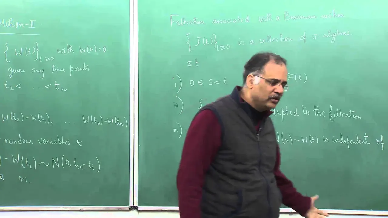




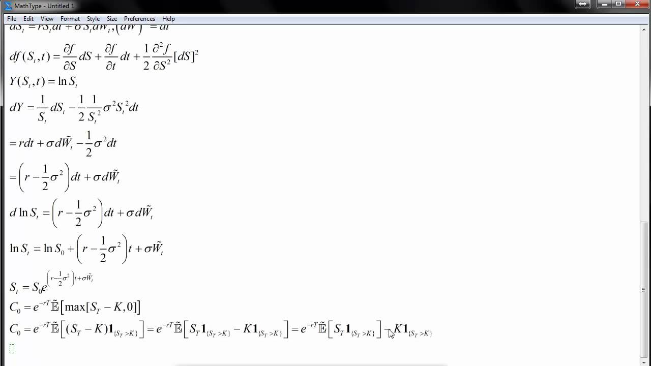





Ito's Lemma is derived by applying Taylor's theorem to a function of time and a stochastic process, then substituting the stochastic differential equation dXt = μt dt + σt dBt and using Ito's multiplication rules (dt×dt=0, dt×dBt=0, dBt×dBt=dt), resulting in the formula: df = (∂f/∂t + μt ∂f/∂x + ½σt² ∂²f/∂x²)dt + σt ∂f/∂x dBt, which provides a method for differentiating functions of stochastic processes.
Deriving Ito's Lemma Using Taylor Series Expansion
Added:Multivariable Calculus and Taylor Series: Understanding how to approximate differentiable functions of multiple variables using partial derivatives.
Foundations of Brownian Motion (Wiener Process): Grasping the properties of standard Brownian motion, including its variance scaling and the heuristic rule that (dW)^2 behaves like dt.
Basic Differential Equations and the Chain Rule: Familiarity with standard calculus chain rules and ordinary differential equations.
Derivation of the Black-Scholes Formula: Applying Ito's Lemma to Geometric Brownian Motion to model stock prices and price financial options.
Solving Stochastic Differential Equations (SDEs): Using the lemma as a stochastic integration tool to solve models like the Ornstein-Uhlenbeck process.
Girsanov's Theorem and Change of Measure: Transitioning to risk-neutral pricing and advanced martingale theory in continuous-time finance.
Stochastic Optimal Control: Exploring how Ito's Lemma integrates into the Hamilton-Jacobi-Bellman (HJB) equation for dynamic portfolio optimization.
50.2K views539likes26:02Original Release: 2016-03-30
hello so if you remember in the last couple of videos we've been building up to this point here um and this point here we basically you at the end of the last video we came up with this um formula which is dxt so where XT is a stochastic process or a random variable to you and me okay and likewise ZT and YT are also stochastic processors or random variables okay and basically we came to this point here and how we got that it was basically the whole idea was we're trying to integrate we're trying to integrate some random variable uh we're trying to integrate some random variable um and we had to do it you can't do it using ordinary calculus you have to do it using this thing called stochastic calculus um and essentially you know the whole point is that YT is kind of looking something like this it's brownie in motion okay so we had to kind of come up with a way of trying to of trying to kind of represent that in a way that we could differentiate or at least represent it in a way that we could represent the process and then try and work with that um and this is essentially what this formula is saying so if you remember we started off at the very beginning we started off looking at a constant function so the random variable is a constant function so in other words Ys is just some constant function okay and looks at how we can integrate that because obviously if we can integrate something then we can just differentiate because it's just a reverse process and integration is just the area underneath that curve okay or underneath that straight line effectively okay then we looked at a slightly more complicated function where we took this um this this idea of a constant okay and just said well actually Ys is just a step function and a step function or step function is just a series of these constant um of these constant functions like we were considering before so we kind of building on the on the idea of just a of just the random variable as a straight line now we've got a straight line which kind of varies okay and then we kind of looked at then the next thing we looked at was how to kind of approximate or if a random variable was looking like something like a well behaved function to like which we're familiar with then we can just use ordinary integration to kind of find that and we call that reman integration so instead of having there a Brownian motion on the end if it's a World behave function essentially we can just have it as um f of s which is our world behave function with respect to S it's just an ordinary integration find the area underneath the curve as we would normally okay and then finally in the last video what we were looking at is basically if we have a brownie in motion something like this brownie in motion what we can do is put it all together put it all together and try and effectively approximate try and approximate this kind of jagged motion this Jagged motion but basically a series of Step functions so you know you series of Step functions effect ly and basically the idea is that we take more and more step functions we get a better approximation of the function get a better approximation of the function so we just basically build this function out of Step functions and that's basically the idea behind you know this this thing here that's how we got to this thing here well what I now want to do what I now want to do here is basically come up with a formula for this because remember this is this is just um what we're saying here is that with the derivative of stochastic process well we can't actually differentiate a stochastic process so this thing here is actually it's it's not meaningless as such because it's a good representation of a of a differential form so we can write in differential form but it actually we can't do anything with it at the moment as it stands we can just say well okay the derivative of stochastic process is this so basically one stochastic process here or random variable here plus another random variable um associated with Brownie and motion okay and this brown in motion term is causing us a lot of issues so basically we can't repres you know this is just a representation of the of the of the differentiation of a stochastic Pro process so we've looked at the integration okay then we managed to get back to the differentiation and this is where we're currently at uh the course so what I now want to do currently at with eos's with eto's integral so what I want to do now is basically look at this this is by the way something called etos Lema this thing in the Box this called etos Lema what I want to do now is I want to look at this and I want to kind of produce some kind of formula for this some kind of formula for this so basically you know okay we can't necessarily do much with it but we can represent presentent it so basically I want to come with a formula that allows us to represent the derivative of a stochastic process okay and that's what we're going to do in this video and in order to do that I'm going to need to introduce this thing called tailor um Tailor's theorem now if you remember we have talked about Taylor's theorem before we have talked about Taylor's theorem before um okay or at least I have done it in other video so if you're interested go please feel free and go ahead and have a look at them I will put them in this playlist uh for you to have a look at um kind of both the derivation and also the visual interpretation of it so I really recommend you do it so for the one variable case Taylor's theem go away Taylor's theorem is f ofx so the function of one variable can basically be approximated by a power series approximated by a power series and if we do it around the point around the origin then it's nice and easy because it's just going to be this so it's the function evaluated at zero okay plus the derivative of the function evaluated at 0 time x okay so now we're getting into involved into the power series because we're introducing an X plus the second derivative of the function evaluated at0 over 2 factorial so that's now a coefficient time x^2 okay and we can basically carry on going so the next one would be uh third derivative of the function evaluated at Zer over 3 factorial Times by X cubed okay and so on so on so on so basically this is just an approximation of the function um as written as a power series and that kind of makes sense because you know in general when we're dealing with functions um we'll have say like you know if you consider a quadratic or a cubic let's consider a cubic you'll have some coefficient times x cubed plus another coefficient * x^2 plus another coefficient time X Plus just a constant term on the end and this is exactly what we've got up here just written around the other way just written around the other way because now the D is if you like just this constant term here okay this CX is if you like this term here okay this BX s is this term here and then if we carryed on going basically we could keep carrying on going so basically what the idea is that we can approximate some function like this um and this is really useful for approximating some function say like which isn't normally written like this so obviously would be no use for a cubic function or quartic function or quadratic function which is already written like this but it would be useful to use something like a COS function or an exponential function or S function or tan function something which does you know say for example if you have f ofx equals cos x yeah the idea is that we can then represent that as a power series like we would in the same way as X squ and whatever it just be an infinite power Series so okay that's the one that's the one variable case this is the tailor series of the one variable case Okay um um but there are we can do all multiple dimensions and so in this video we're actually going to consider the second dimension case so in other words we have F of um it's going to be F of XY okay um so we're going to have two variables f of x and y so X and Y are the two variable case um and what I'm actually going to do for convenience I'm going to change this to an a the reason why I'm going to change this to an a maybe I'll change this to a b as well the reason why I'm going to change those variables is because I want to basically EV I want to compare it to something later on I want to compare it to eto's Lema and eos's Lema already involves things like X and I don't want you to get confused so I'm going to call it a and b okay but effectively you know it's just any two variables so I evaluate the function at zero again the origin okay plus the first derivative of the function and the derivative of the function with respect to the first variable der to the function with respect to a and evaluate that at 0 0 okay uh Times by a okay so Times by a Times by my first variable and then I do so basically here I'm just considering all the possible combinations of first variables uh sorry first derivatives so I can differentiate my function with respect to a but I can also differentiate my function with respect to B so in other words F of B 0 0 times B okay so I've done all the combinations of first derivatives now I'm going to do all the combinations of second derivatives okay so the first all the combinations of second derivatives I'm going to end up with plus F I can have second so second derivative of a with a and a so um the function differentiated with respect to a twice so f a a and again evaluated at the origin evaluated at the origin okay Times by a s so how I think of it is I look at the the number of derivatives I've taken it with respect to and that kind of corresponds to this so if you're like you know that kind of looks a bit like a squ it's not a squ it's the second derivative of my function with respect to a okay um but I just kind of you know I look at that and I say oh that's almost a squ that's a good way of remembering it okay and I keep that over two factorial okay plus what else can I have the second derivative I can have well I can have the second derivative with respect to B as well have the second derivative with respect to B um so fbb evaluated at 0 0 and again that's over two factorial and again I just look at this BB and I see that's that's pretty much B squ right it's not but it is um and what are the second reative what I can I have well I can have also the derivative of a with respect to B sorry the derivative of my function with respect to a and then with respect to B and I assume that that's the same because it's kind of a nice function that it's the same as the derivative of B with respect to a so those two things are the same and they usually are okay so those are basically you know that's my next derivative so my derivative of my function with respect to A and B evaluated 0 0 and again I look at a * B and I think oh okay that's just a * B there okay so it's Times by a * B and there's no over two factorial here okay effectively the two factor is kind of just cancel out I think plus dot dot dot that's how I think of anyway so that's basically the second a derivative of my function sorry my you know my expansion of my Taylor series with two variables and I'm going to now use that um and try and kind of relate it back to something which looks like this so I'm going to use that as well so so what I want to basically do what I want to basically do is I want to find the derivative of my function my function um of T and XT now what does that mean well it's basically this it's basically basically this because look if I have if I have if I try and plot this graph okay I can have my random variable or my stochastic process XT and that is dependent on time that is dependent on time so in other words I'll have to have t down here so in other words whatever my you know whatever my stochastic process is doing um it's going to be of two variables so this is what basically this means DF and it's going to be of two variables time and also my stochastic process XT okay now here's where I'm going to go in so notice now I've got a D up here I didn't have a d with my tailor series I didn't have a d actually fact I'm going to write out my tailor series again just so then we can compare it to something okay so there's my you know I've written my Taylor series out again now WR my Taylor series out again okay so let's just consider the first term so notice the D here but I'll come to that when when I need to come on to it so notice my first term so my first term is my function evaluated at 0 0 well if T equals 0 if T equals 0 so T equals 0 then what does XT equal so what does x0 equal well we just take its kind of if you like standard brown and motion this is what I'm trying to approximate standard brown em motion and tells me that standard brown motion um at the origin it starts off at zero okay standard brown motion starts off zero so therefore that is zero so F of 0 0 should just be zero my first term should be zero so I just don't bother writing that so basically I don't need to consider that term okay then you consider that term so basically now I'm looking at this term this F of a sorry my function der differentiated with respect to a Times by a what is a now a is now a is now um a is now T okay but it's no longer T this is where my D comes in if you like my D is multiplied by T so I end up with DT okay so I differentiate my function the derivative of my function with respect to T because that's now a okay a is now t b is now XT okay and so it's deriva of my function with respect to T I could write it kind of you know how I've written up here but I'm going to write it like here because I think it would make more sense to you but now I've got my D here I've got to take into account my D here so it's not just T it's D and if you're like you know this is by the way this isn't a proof which I'm showing you this is not a proof that I'm showing you this is just a an idea of why it's true so there's kind of some mathematical fudging it's not like a rigorous mathematical argument it's a bit of mathematical fudging for example this thing here okay because I've stuck a d out the front there so therefore this becomes DT there's no reason why mathematically that should make sense but the point is we know that this works we know that what the formula which I'm going to end up with at the end of this video we know that that works so what we're going to basically do is kind of um you know there's going to be a bit of mathematical fudging along the way this isn't a rigorous proof nobody can actually prove this okay this is kind of the whole idea of financial mathematics well Financial mathematics is sometimes a bit of a wavy argument it's kind of like well it works so why not just use it and it kind of just you know this is this is an argument of why it could make sense but it's not a rigorous mathematical argument so a mathematician kind of is looking at and thinking no obviously not that doesn't make sense mathematically but a financial mathematician kind of say nah that'll do okay so this is effec what we're doing here we're just kind of showing you an argument of why it could work of of why it kind of why why works okay not necessarily a rigorous proof okay so that's that term there so now let's consider this term here it's F of B with respect to B so I've got F of B so I'm going to differentiate f with respect to my random variable and I'm going to actually call my random variable X so XT I'm just going to call it X when I'm differentiating SP to X again it's one of these wavy arguments I mean it does kind of make sense because if you know if you take the probability if you take the probability of a random variable is equal to some value so basically the random Val variable so it's like probability that capital x is equal to X this is a random variable this capital x is a random variable it's basically all the values um that you know we can that X can possibly be and Little X is just some particular value so this is kind of an argument of why we kind of change it to Little X basically just because it works is fine um but if you want a little bit more justification argument but now like I say we just keep this XT now so this is just dxt okay so this is D so my B is XT now okay and I keep that XT I want that XT now just said here I want to change it to X but now I'm going to keep that XT and I'm going to use this D out the front Okay the reason why I'm kind of writing it like this dxt is because the whole idea is I've got an integral okay I've got an integral of something and when I have an integral of something I've got a DT or a dxt okay so this is why I kind of write this dxt here so there is a little bit more going on in the background but for the moment I'm just presenting you with an argument of why it could make sense okay uh so that's that term there so now let's consider this term here so in other words we've got half because that's one over two factorial so I'm going to take care of the factorial first times the derivative of my function or the second derivative of my function with respect to a what was a it was DT so it's dt^ 2 okay and what's a well it's t but remember it's DT okay it's DT and that's all squared because that's what that a squ means okay apparently according to financial mathematicians okay so next term this is this term now I'm dealing with with this term now so I've got the second derivative of my function so half first of all take care of the factorial I've got my second derivative of my function okay with respect to B what was B it was dxt well I'm differentiating so I'm going to change it to Little X so I've got dx2 okay time b^ s so now I'm going to use my now I'm going to use my D XT yeah dxt and I'm going to square that so I've got dxt ^2 now Okay cool so I've got that now oops I've got that now okay then finally my last term which I'm just going to consider is the derivative of my function second derivative of my function with respect to a then with respect to B so in other words with respect to T with respect to T then with respect to x with respect to X X and I've got then an AB be multiplied at the end so my ab is T So DT time x dxt dxt this is what I end up with and then I can carry on going like that now we can do a bit of simplification we can do a bit of simplification right um because basically if I just pull up this table uh and again I'm reluctant to pull up this table but I have to pull up this table for this step um but I'm going to have to justify why I'm not going to using this table in just a moment um basically basically this table if you remember this multiplication table which I introduced think the last video maybe the video before I think it was the last video um where basically If I multiply DT by DT I get zero If I multiply DT by dxt I get zero multiply DT by dxt I get zero If I multiply dxt by dxt so in other words dxt 2 I get DT okay so basically anywhere I see DT by DT or DT squ like here for example I see DT dt^ S I should get zero so this becomes zero so therefore this term just goes away okay and likewise whenever I see a DT by dxt like I do here for example that goes to zero so other words this term goes away so in other words what I'm left with so if I now get rid of that okay and you could argue you know you should have I tried to get away with it but I will kind of own up now this should be you're saying oh you're saying that dxt 2 should be DT yes it should but I'm not going to do that for the time being because actually if I do that then I I miss a term this is like I say you know this is like a it's not a rigorous mathematical argument at all okay this is just a reason this just a I'm just tring to show you suggest why why it could be true so what am I left with I'm left with the derivative of f with respect to T time DT okay got that term um plus the derivative of f with respect to x times dxt so in other words that term okay plus the only other term I've got left is that term and by the way all of the these plus plus plus plus you know all of these other minuses plus and minuses I will get something like DT by dxt or dt^ s or DX you know T by DT so in other words all of these terms will go to zero actually quite nicely so all these what's known as higher order terms so in other words you know if I considered if I kept on expanding this out they would all have either a DT by dxt in or a DX or DT squ or something like that okay in there so therefore it would all go to zero okay so what am I left with half D2 F by dx^ 2 oops dx^ 2 times by dxt all squar now basically the idea is the idea is this tailor expansion um should be described by this tailor expansion should be described um by eo's L or EOS LMA should be described by this tailor expansion okay so in other words etos Lema which is dxt um is equal to ZT DT plus YT DBT okay that should be described by this EOS Lema which I've got written up here so if I just shift this over a little bit okay to make a little bit room over this is d f of txt okay this is describing that in other words so basically these two things these two things are exactly the same or rather you know this thing is same as this thing yeah so other words those two things are the same this is basically a tailor expansion because this is just exactly describing that you know I tried to justify that by using the graph you know this is a stag gastic process and it changes over time so therefore there's going to be some function in here and that function is going to be approximated by here by this okay excuse me okay so what I want to basically do what I can do then is I can make some substitutions for this in here okay so in other words whenever I see a dxt like I do in here and like I do in here then I can just make a substitution so this substitution is nice and easy because it's just that okay so in other words I can say that D DF of txt is equal to this term is left alone I can't make any substitutions there or any meaningful substitutions there plus the derivative of f with respect to X okay times dxt so in other words if I replace that in there okay other words if I repl that in there so I end up with ZT DT plus YT DBT okay so I've replaced that in there plus a half of the second derivative of f with respect to X okay plus this Times by this thing squared so in other words now if I sub that in there and square it so basically what I'm going to ask is let's just ask what is dxt squar so in other words this thing what is this thing squared well let's have a look ZT DT plus YT DBT okay multiply that by the same thing so ZT DT plus YT DBT oops BT DBT so let's just expand this out this is just basically a quadratic right so we end up with ZT multiplied by that thing so we end up with zt^ squar multip by dt^ 2 okay so that's that thing Ted let's do then this thing multiply by this thing so plus ZT YT DT um Times by DBT and if you notice that when we do that times that we get exactly the same thing so it's going to be plus two lots of that okay plus two lots of that um and the last thing we got to do is that multiply by that so plus YT squar yeah plus yt^ squ got YT YT yt^ 2times DBT s DBT s now this is when I pull up my table again so I've got my table this is DT this is DBT same thing on the top DT DBT BTT this is zero DT squ is zero this thing is zero this thing is zero and this is DT so other words this thing which is a DT DT squ that's zero okay so that goes away okay this thing which is DT multipli by DBT is zero from this thing here so therefore that goes away and DBT just turns to DT so what we left with what we left with we're left with dxt dxt should just be equal to YT ^2 multip DT okay so now I can sub that in for dxt ^ 2 so dxt ^2 is just that thing so yt^ 2 DT yt^ 2 DT okay and then basically I can just do a little bit of um expansion so let's just get rid of this to make this make a little bit more room okay so basically now it's just a case of simplifying this so I'm just going to expand this out okay so we end up with this is equal to the partial derivative of f with respect to T DT okay plus parti derivative of f with respect to X multipli by ZT DT uh plus partial dtive of f with respect uh respect to X multiplied by YT DBT so I'm just multiplying this thing out now okay and then I've still got this thing added on the end so plus half second root of f with respect to x^2 YT ^2 DT okay so that's that thing simp that's that thing expanded out then basically look we've got a DT here DT here and a DT here so let's let's let's take out a DT out this thing so DF by DT okay so that's that's going to go inside my DT bracket my DT bracket okay what else is going to go inside my DT bracket this thing's going to go inside it so plus DF by DX X ZT okay what else is this thing is as well so plus a half second root of f with respect to x s yt^ 2 okay and what have I got left over I've just got that term left over on the end so other words that thing left over on the end let just a little bit smaller shift over um change that to nice Delta there we go plus second derivative of f with respect to X YT DBT okay so basically now I can represent my function so by DFT so DFT uh let's make this still a little bit smaller so I can fit my DFT in come on okay so there we go so that is my final that is my final formula so now I can represent my ETO process or my etos Lema like this okay so now basically when I'm when I'm trying to differentiate stochastic function I basically can represent it like this okay okay and that is it okay I can represent it like this but I can't necessarily do anything with it this is kind of um you know in this course at least we can't do anything with it we can just represent it like this so that I can just say that my derivative of my stochastic process is given by this there is a nicer simpler way which I can use it which I kind of used up here we're basically all simple way of writing it if you like so rather than writing you know dxt all the time I can just write this is this is f yeah so I can just write um f with respect to T f with respect to T so this is just shorthand way of writing it using subscript notation F subscript T just means the derivative of f with respect to t plus and I've got f with respect to x * ZT okay plus a half half of my second derivative of f with respect to X so FXX yt^ 2 okay that's all multip by DT plus f with respect to X YT uh DBT so perhaps that might be a simpler way of remembering it know but they're both the same it's either way that you want to remember it that's fine
Up Next

9:44
Geometric Brownian Motion Explained: Stock Prices & Log-Normal Distribution
@MathPartner
78.4K views•2016-03-29

4:43
Elliptic Curve Cryptography Explained: ECC, ECDSA, ECDH
@PracticalNetworking
28.5K views•2024-10-21
28:34
Brownian Motion from Random Walks: A Mathematical Derivation Guide
@MathPartner
49.8K views•2016-03-28

6:00
The Mathematical Impossibility of Accurate World Maps
@Vox
23.3M views•2016-12-02
Related Study Plans & Knowledge Roadmaps
Structured learning paths in Mathematics
mathematics
Tensor Calculus: Vectors to Riemann Curvature
01Mathematical Foundations: Linear Algebra & Calculus
02Covectors, Dual Spaces, and Tensor Basics
03The Metric Tensor and Index Gymnastics
+ 2 more learning modules
40h5 modules
Explore Roadmap
mathematics
Gödel's Incompleteness: Logic, Proofs & Limits
01Introduction to Formal Systems & Hilbert's Dream
02Set Theory, Cardinality, and Cantor's Diagonal Argument
03Arithmetization and Gödel Numbering
+ 2 more learning modules
14h5 modules
Explore Roadmap
mathematics
Galois Theory: Fields, Groups & Solvability
01Foundations of Abstract Algebra: Groups & Fields
02Polynomials & Field Extensions
03Splitting Fields & Symmetries
+ 2 more learning modules
24h5 modules
Explore Roadmap
mathematics
Non-Euclidean Geometry: Models & Geodesics
01Euclid's Fifth Postulate and the Birth of New Geometries
02Hyperbolic Space and the Poincaré Disk Model
03Geodesics: Defining Straight Lines in Curved Spaces
+ 2 more learning modules
15h5 modules
Explore Roadmap