Geometric Brownian Motion Explained: Stock Prices & Log-Normal Distribution

[00:00:00]Hello. So, in this video, we're going to be talking about this thing called geometric brownie in motion. Okay. And so, what we're going to actually try and do is apply brownie in motion um to kind of share prices or asset prices um in finance in financial derivatives. Okay.

[00:00:15]Um so, basically we presume that a share price a share price will basically follow this kind of brownie in motion.

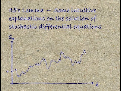
[00:00:22]So, what we want to try and do is come up with this brownie in motion. So basically a share price we would expect a share price to kind of grow in an exponent in an exponential manner because obviously the more shares that you've got uh or as you go forwards in time you know say if your share price is doubling each time okay then obviously that's going to be an exponential manner you know it will follow some kind of exponential graph. basically you know if this is share price against time so the value of your share against time it should follow some exponential manner it should grow exponentially okay uh and this is you know your start price snort so basically it's going to start at snot and it's going to grow um by some factor over time an exponential factor over time this is just your standard you know exponential growth um you start at snot okay you grow exponentially over time by some factor alpha okay and that's what's going to that's effectively where where um where where share price you know share price basically wants to grow in this way but of course we know we know that share price and well I can just tell you that share price follows this thing called brownie in motion so therefore we need to basically include some kind of brownie in motion um into it and in actual fact you know brownie in motion so in other words it's going to grow in this way but effectively there's going to be kind of you know it's going to grow um with this kind of jagged motion it's not going to grow in like one neat smooth little curve. So effectively that brownie in motion comes in. It's going to, you know, it follows the same kind of shape as the standard exponential graph. You know, the standard exponential graph, but the jaggedness comes because it follows an follows brownie in motion. Follows brownie in motion. Okay? So we're going to have to take into account that brownie in motion. Okay? And we just take into account with it uh with an extra term. So in other words, it's brownie in motion um times some constant effectively. And that constant is known as beta. So it's beta times some constant. beta you know it doesn't really matter what that value of beta is uh in actual fact you know there is it's uh it's very difficult to measure what beta is um but yet it's very very important okay it's very very important um in fact whole industries in finance are dedicated to measure what this value of beta is but for the time being if you can just kind of spot well okay this is this is an exponential growth okay plus some kind of ex this term here just contributes to the um the brownie in motion okay this kind jaggedness to it.

[00:02:40]And if you just understand that for the time being, then that's absolutely fine.

[00:02:44]That's absolutely fine. Okay.

[00:02:47]Um Okay. And actually, this is the share price at strictly speaking, it's the share price. Go away. This is the share price at some time T. So, we actually call it S S little T. That's just simply the share price at some particular time.

[00:02:59]Okay. So, it depends on T. Right. Now, let's try and fiddle this. Let's try and fiddle this. Um Okay. Okay. Let's try and fiddle with this. So I'm going to divide by S. So I'm going to end up with ST over S equals E to the alpha T plus beta BT. Yeah, going to end up with that. Um then let's get rid of this E.

[00:03:22]Let's get rid of this E. Um and let's just take the logarithm of both sides.

[00:03:27]So that implies that the logarithm or natural logarithm of ST over SN equals alpha T plus beta BT beta BT. Okay, so that's what that equals. Now this term here, this term here will contribute to the mean.

[00:03:44]This contribute will will contribute to the mean. So it contributes to the mean.

[00:03:48]Okay, this term here and this term will contribute well this term basically basically means that the mean is zero of this term.

[00:03:57]mean is zero. Um and so basically if you try and model if you try and model alpha t plus beta t beta bt beta bt um that is kind of exponential you know that is kind of if you remember if you remember that um bt brownie motion is normally distributed under standard normal distribution uh sorry under standard brownie motion uh brownian you know which is what we're considering brownian motion is distributed by a normal distribution of mean zero and variance uh t okay variance t okay but now so how will this so basically what I'm trying to do is write this in some kind of you know it's very very close to this you know this this here is very very close to this bt is normally distributed understand normal distribution okay so basically I know it's going to be normally distributed but what's going to happen what's going to happen um well this term here tells me that the mean is going to be zero because it's standard brownie in motion. So therefore, the mean is going to be zero.

[00:05:01]Okay? But so this term here, the mean is zero, but I'm adding to that I'm adding to that an alpha t. So if you like, I've got zero plus my alpha t. Okay? And likewise for my variance. So therefore, this this is just going to become alpha t, right? This is going to become alpha t. So then what's my variance doing?

[00:05:18]Well, my variance is going to be t, but it's going to be multiplied by some constant. And that constant is my beta.

[00:05:25]that constant is my beta because you know I've got my BT here, got my BT here. Adding alpha t to my variance is not going to make a huge bit difference because remember variance is just the amount of spread. So the alpha t if you like is just translating you know my terms. It's not going to affect my spread spread. It's not going to you know affect my spread by any means. If you like you know my variance between two points say if this is this is like three and this is seven for example. I know it's really contrived example but then say for example if I add if I add some terms so let's say for example if I add two to it then this term is just going to be moved to here so it's going to be moved to five and this term is just going to be moved to here it's just going to be moved to nine okay so now I'm just considering that so it's not going to affect the spread it's going to be exactly the same spread effectively but multiplying it by beta so it's going to be t but multiplying it by beta is going to make a huge difference because I'm basically going to affect the variance how's it going to affect it well it's not going to affect it beta it's going to be vectored by um beta squ because if you remember if you multiply a random variable by a constant if you find the variance of it then it's just going to become that constant squared then okay go back to your kind of second year so basically what I'm saying is the variance of if you have the variance of x say for example okay um is equal to I don't know is equal to yeah okay let's say that's equal to no I don't want to say that that's equal to a okay then the variance of k * x okay is going to become k^ 2 * a okay so it's going to affect it by by you know square basically so this is now what it becomes this is quite a messy isn't it let me write it out below so I've got basically alpha t alpha t plus betat t is normally distributed normally distributed by a mean of 0 plus alpha t so alpha t um times beta 2 * t if you at least half followed that then well done quite frankly um because you know you don't need to kind of understand the ins and outs of it but if you can at least half understand at least kind of see where things come from I think it makes a huge difference uh but of course this alpha t plus beta t what was that equal to that was equal to natural logarithm of s t over s so I can just replace this with the natural logarithm of s t over s okay that's normally distributed by alpha t beta^ 2 * t Okay, so that's basically what we end up with and this is what's known this is what's known as log normal. So in other words, we can say that the ratio of the share prices, so this is a share price at time t compared to the share price at the beginning. So the ratio of the share prices is what's known as log normal. The reason why it's called log normal, I wonder if you can guess. We've got a normal distribution there and we've got a log there. So we put the two together, we got log normal.

[00:08:12]Okay, log normal. Okay, and it's a logn normals curve. So let's have a look at the log normal curve. So this is a log normal curve. Okay. Well, what's a what's a normal curve going to look like? Well, a normal curve a normal curve is just going to look like this. It's just going to look something like this. It's a bell-shaped curve, right? Uh but the log part just basically means that it's skewed. It just makes it skewed. So it's a bit like a stretch. So it's going to effectively look like this. Okay. So that's what a log normal curve looks like. It's just a it's a normal curve but just skewed. Okay. um and we go through the origins. Okay. So, what is now geometric brownie in motion going to look like? Geometric Brownie motion, GBM for short. Well, I've drawn it above.

[00:08:52]I've drawn it above. It's just this graph here. So, we know we know that the um we know that the you know, if I just write S= S or ST= SN E to the alpha t, I know that that's going to look like this. I know that's going to look like this. Okay. And then if I plus a brownie in motion term, then that's when I get my kind of jaggedness. So this is what geometric brownie in motion effectively looks like. Okay, so it's exactly the same as what I've just drawn in there.

[00:09:20]Right? So the spikes is just contributed by the beta bet. Okay. Um and this really is fundamental quite honestly.

[00:09:28]This is fundamental um to kind of um you know geometric brown motion is really fundamental in everything that you're going to do from this point forward.

[00:09:37]Okay, I'm just going to talk about brand geometric brand motion.