



















Geometric Brownian motion is a stochastic process used to model stock prices, where the logarithm of the stock price follows a normal distribution with mean μt and variance σ²t; it can be simulated in Python using numpy by calculating the drift term (μ - σ²/2) × dt, generating random normal samples scaled by √(dt), and applying the cumulative product to accumulate changes over time, with the final stock price given by S₀ × exp[(μ - σ²/2) × t + σ × W(t)], where W(t) represents the Brownian motion component.
Simulating Geometric Brownian Motion in Python | Quantitative Finance Tutorial
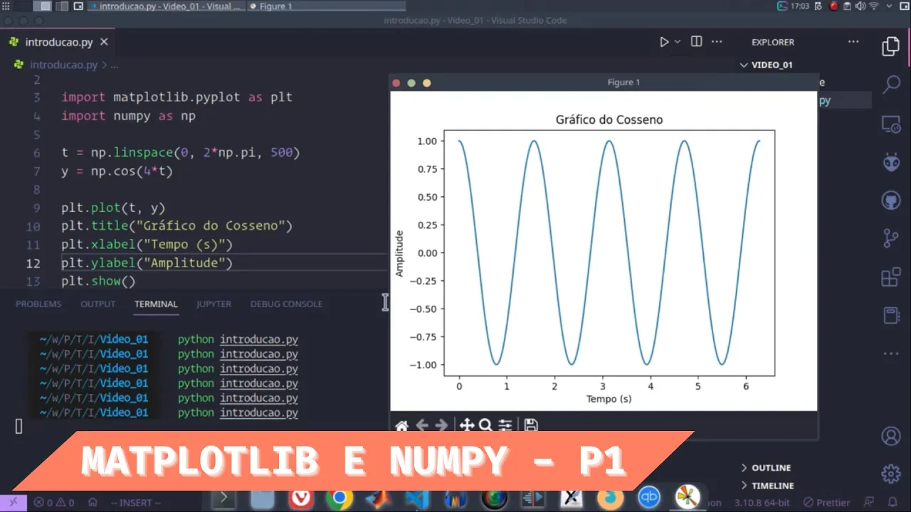
Added:Intermediate Python programming skills, particularly using scientific computing libraries like NumPy for array operations and Matplotlib for data visualization.
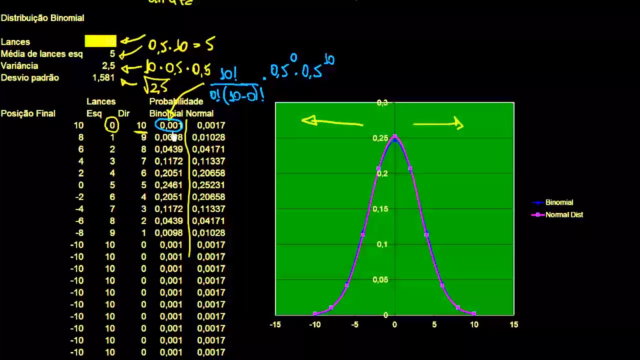
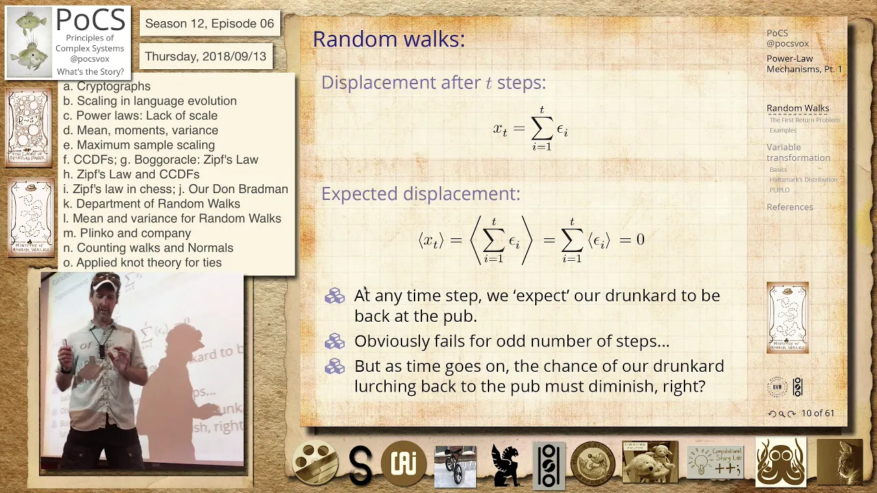
Basic probability and statistics, specifically concepts like the normal distribution, random walks, and mean/variance.
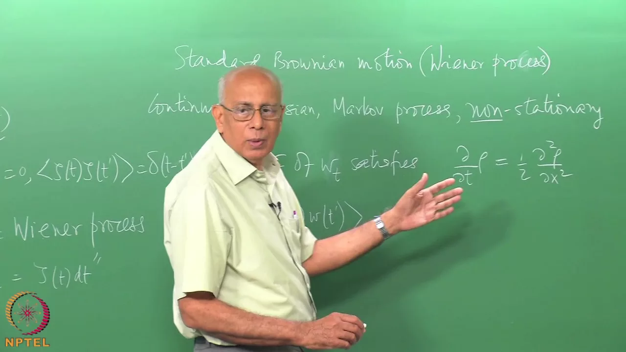
An introductory understanding of continuous-time stochastic processes, particularly the standard Brownian Motion (Wiener process).
Fundamental quantitative finance concepts, such as asset returns, drift, volatility, and the assumption of log-normal stock price distributions.
Applying simulated Geometric Brownian Motion paths to price derivative contracts using Monte Carlo simulation (e.g., pricing European Options).
Parameter estimation and calibration techniques to extract historical drift and volatility parameters from real-world financial market data.
Exploring more advanced stochastic asset pricing models that address the limitations of GBM, such as the Heston Stochastic Volatility model or Jump-Diffusion models.
Implementing financial risk management frameworks, such as calculating Value at Risk (VaR) and Expected Shortfall (ES) using simulated portfolios.
44.4K views992likes8:48Original Release: 2021-09-15
g'day youtube and welcome back to the asx portfolio channel my name is jonathan so today we're actually just going to be simulating geometric brownian motion in python we're not going to be going through how to derive these dynamics but we'll be doing that in the following tutorial and we'll be understanding ido calculus ido integrals and understanding stochastic processes so if you want to learn more about that please subscribe to the channel and hit the notification bell so you can see that video when it comes through so let's jump into simulation so i'm going to be going through this jupiter notebook here so here we have geometric boundary motion we have an initial stock price which is greater than zero and the dynamics as defined by this stochastic differential equation so here we have a couple of terms we've got this mu which is the coefficient for drift we've got a constant coefficient for volatility as a percentage point which is sigma and then we have this drift term and then the actual stochastic uh integral component which is this ito integral um which has this brownian motion component so here in integrated form you can see that the log of the stock price follows this normal distribution um with respect to this drift the initial stock price and then it has a variance that's defined by this sigma squared with respect times by the time so in explicit form in explicit form we have the initial stock price exponential to the power of these two terms here so let's just get ahead and actually import our dependencies so for this we're going to need to import numpy numpy as np and we're going to import matplotlib dot py plot as plt so now that we've got that let's define our parameters so our mu is going to be 0.1 or 10 over a year time horizon our number of time steps is what we're going to define as n now let's just say a thousand that should 100 that'll give us granular piecewise simulations so we can view that on the graph let's go time in years so big t that'll be one number of simulations let's call that m and we'll give a hundred initial stock price s o which we can call a hundred and volatility which we'll define as sigma and we'll call that 30 so run that now the simulating the geometric brownian motion paths so first off we need to calculate the actual time step um because we want to return a vector for all these paths for all these time steps so let's calculate that that'll just be t divided by n really simple now let's use simulation using numpy arrays we're going to do this in one step instead of iterating over for paths so let's call this st now we're going to go numpy exponential now within this function here we're going to do these components so mu minus sigma to the power of 2 divided by 2 that'll be times by dt now that we've got that component we need to go sigma times by numpy array let's just put some spaces in here so you can really see this clearly times numpy array and that'll be random dot normal so we're going to be randomly sampling from the normal distribution and that'll be np [Music] square root with respect to that dt so we're just going to be randomly sampling from brownian motion with a the square root of that change in time for each time step now the size of this is going to be the number of simulations by the number of time steps we want to take now because of the form that we want this in um we're going to take all of this we're going to take the transpose of this random normal so once we've got this time step we want to take the transpose so that we're actually getting the simulation for each time step so once you've done that what we need to do is actually include a initial point an initial ray of ones and you'll see why in a second so we're going to use v-stack for this so it's just numpy v-stack and all you need to do is call numpy ones and the dimensions that you want is the same as our simulation number so 100 that's m and we're just combining that with the st simulation numpy array so once we've got this stacked together all we need to do is multiply this through by our initial value and what you'll notice here is that this is the daily or the time step changes in terms of the drift and then the variance and the stochastic component so this is the time step implementations and what we need to do is actually accumulate these over time so we're going to use the cumulative product along each simulation path which is axis 1 so for that what we need to do is actually multiply this by st and we're going to use this function called prod so we need to define the axis of which it's going to calculate the cumulative product and that's going to be axis 1 which is across each of those simulation paths so once we've done that we can hit enter the yeah we can probably view one of those stacks now so let's just return that array and you can see here's a simulation path for time step one so now let's consider the time intervals in years so what we need to do is actually use numpy space for this so we're only going out to one year but we have need evenly spaced time steps so to t and we're going to have n plus one spaces so this will get us back an array and let's just call that t or time and then now we need to require a numpy array that is the same shape as st and we're going to use that so we can plot the function so all we need to do is go np dot full so we're creating a a shape that is the same as our st array which is m n plus 1 now it was m n but now we actually added the array of ones so now that is going to be m n plus one and then we're going to fill this entire value so our fill underscore value is going to be equal to time so i'm just going to have an array for each of these simulations that's just equivalent to the time so we're going to take the transpose of this vector now and we're going to run that so now we can plot this graph and you can see here that we have years along the x-axis we've got the stock price along the y-axis here we've got our dispersion resulting from the 30 volatility and our 10 increase in the the mean the drift over this um geometric brownian motion so hopefully you guys learned a lot on just how to simulate geometric branding in motion but yeah in general geometric branding motion is a very useful model for option pricing theory and um i hope you get a lot of value out of this tutorial in the next one we're going to learn okay how can we actually use financial mathematics eto calculus ido integrals and understand that so we can then start increasing the complexity of these stochastic differential equations to try and add different parameters so if you want to learn more about that jump and jump into our next video next week hit the notification bell so you're notified when that comes through anyway until next time youtube see you later
Up Next

12:43
Solving Stochastic Differential Equations | Asset Pricing
@uchicagoonline8873
61.7K views•2016-06-22

4:43
Elliptic Curve Cryptography Explained: ECC, ECDSA, ECDH
@PracticalNetworking
28.5K views•2024-10-21

10:44
Fourier Series Introduction: The Big Idea Explained
@DrTrefor
387K views•2021-05-03

6:00
The Mathematical Impossibility of Accurate World Maps
@Vox
23.3M views•2016-12-02
Related Study Plans & Knowledge Roadmaps
Structured learning paths in Mathematics
mathematics
Tensor Calculus: Vectors to Riemann Curvature
01Mathematical Foundations: Linear Algebra & Calculus
02Covectors, Dual Spaces, and Tensor Basics
03The Metric Tensor and Index Gymnastics
+ 2 more learning modules
40h5 modules
Explore Roadmap
mathematics
Gödel's Incompleteness: Logic, Proofs & Limits
01Introduction to Formal Systems & Hilbert's Dream
02Set Theory, Cardinality, and Cantor's Diagonal Argument
03Arithmetization and Gödel Numbering
+ 2 more learning modules
14h5 modules
Explore Roadmap
mathematics
Galois Theory: Fields, Groups & Solvability
01Foundations of Abstract Algebra: Groups & Fields
02Polynomials & Field Extensions
03Splitting Fields & Symmetries
+ 2 more learning modules
24h5 modules
Explore Roadmap
mathematics
Non-Euclidean Geometry: Models & Geodesics
01Euclid's Fifth Postulate and the Birth of New Geometries
02Hyperbolic Space and the Poincaré Disk Model
03Geodesics: Defining Straight Lines in Curved Spaces
+ 2 more learning modules
15h5 modules
Explore Roadmap