



![[Fall-2022] Tutorial: Probability](https://i.ytimg.com/vi_webp/rcXeRCGCh4o/maxresdefault.webp)




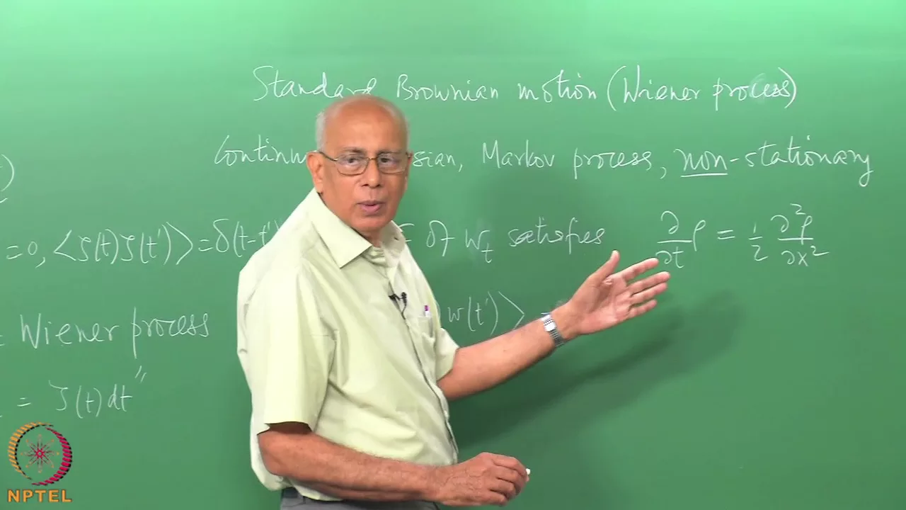

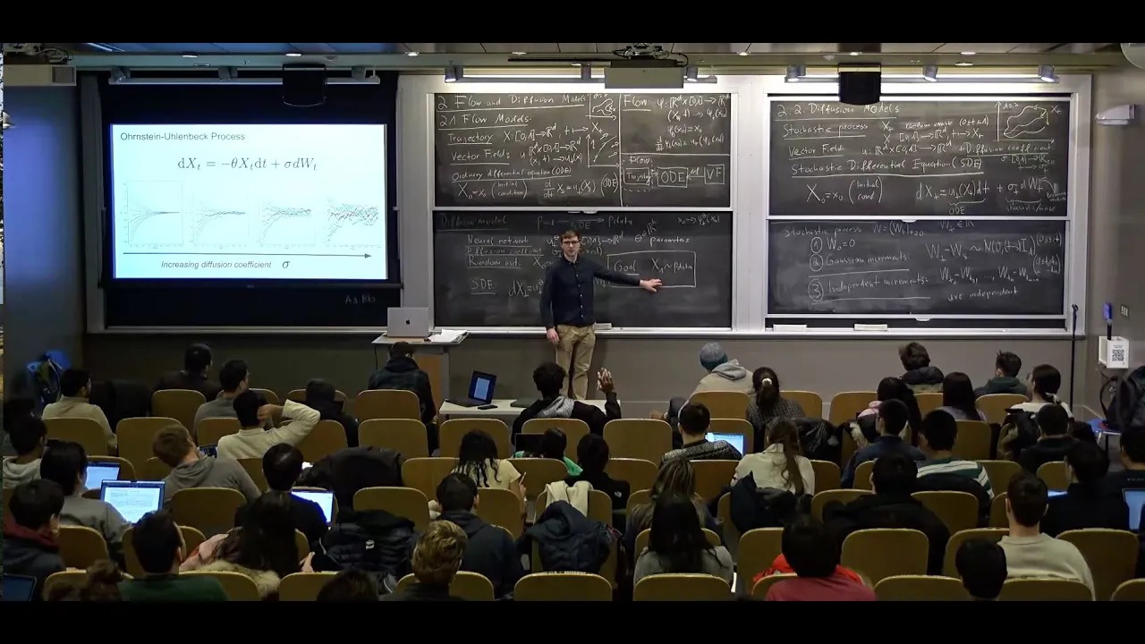











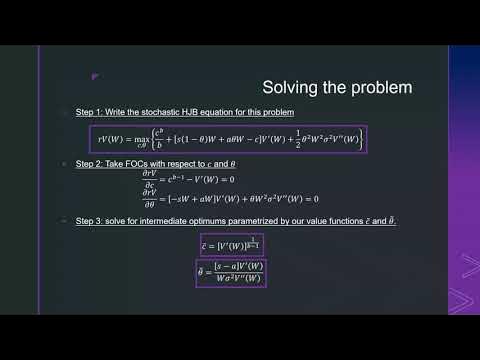


Solving stochastic differential equations involves integrating both sides of the equation to express the solution as the sum of deterministic components and stochastic integrals; for example, the solution to dX_t = μdt + σdZ_t is X_T = X_0 + μT + σ∫dZ_t, where the stochastic integral ∫dZ_t represents a normally distributed random variable with mean zero and variance T, and this approach extends to more complex models like geometric Brownian motion for asset prices, which yields log-normally distributed prices.
Solving Stochastic Differential Equations | Asset Pricing
Added:Foundational ordinary differential equations (ODEs) and basic calculus-based integration techniques.
Core probability theory, including random variables, expectation, variance, and continuous probability distributions.
An introduction to stochastic processes, specifically the definition and properties of a Wiener process (Standard Brownian Motion).
Basic financial economics concepts, such as asset returns, discounting, and the time-value of money.
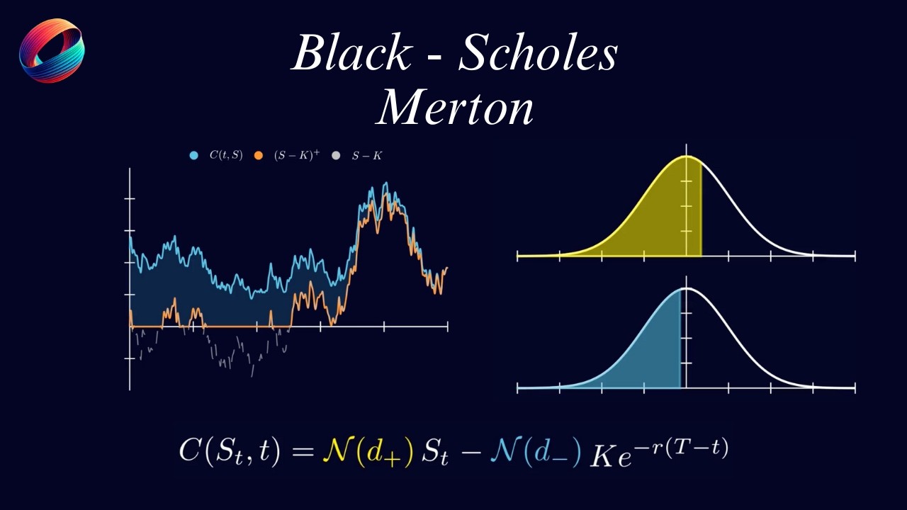
The Black-Scholes-Merton option pricing framework, which directly applies Geometric Brownian Motion to value financial derivatives.
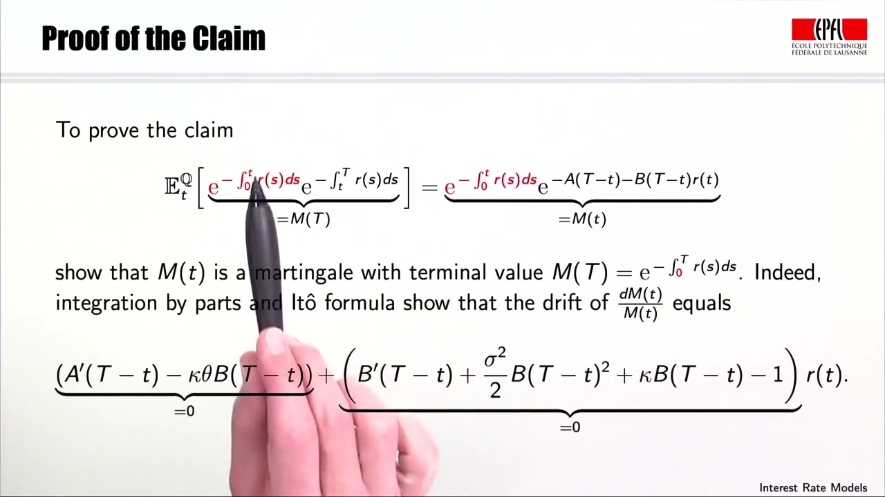
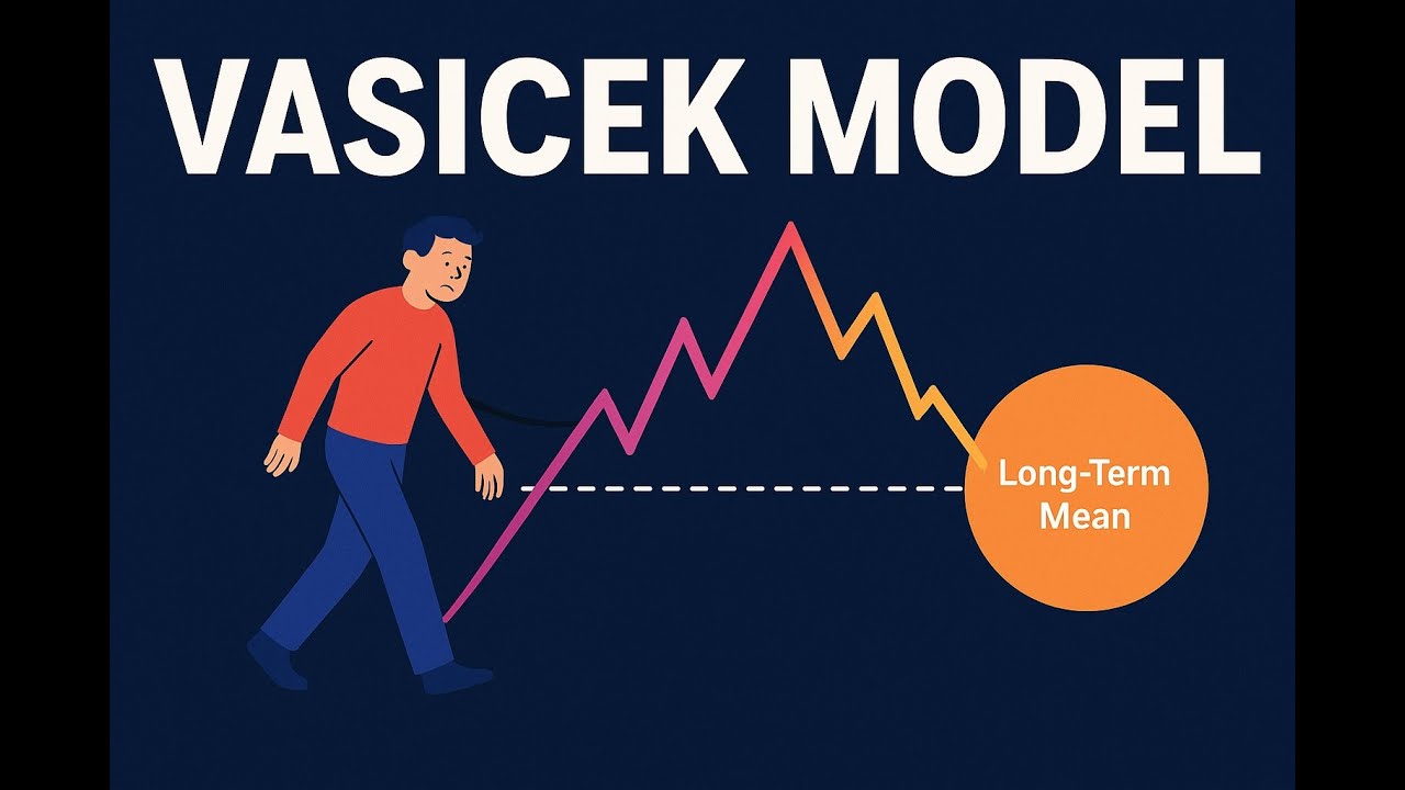
Advanced interest rate models using mean-reverting SDEs, such as the Vasicek and Cox-Ingersoll-Ross (CIR) models.
Numerical simulation methods for SDEs, including the Euler-Maruyama approximation scheme and Monte Carlo pricing techniques.
Continuous-time portfolio optimization and asset allocation models, such as Merton's portfolio selection problem.
61.7K views658likes12:43Original Release: 2016-06-22
[Music] welcome back this is our third and last video on stochastic calculus and continuous time methods now we're going to talk about solving stochastic differential equations a forbidding title but actually an a interesting and fairly simple idea you've done this in discrete time in discrete time we started with a stochastic difference equation uh the ar1 and you know how to solve the ar1 meaning Express today's X in terms of the long uh distant past and all the sequence of shocks that's just the the anti-derivative if you will of this that's the differential form that's if you will the integral form our job is to learn how to do exactly that kind of operation with the kind of diffusion processes that we've been talking about so let's start with the simplest one the stochastic integral we originally defined DZ as the difference of the Z process now we want to go back and do the corresponding integral of the differential that we took the first time around so if you have ZT and you want to go back to the level why don't we just say that the level of Z is the integral of all the changes that's what we do in discreete time in discreet time the level of Z is just the sum of all the changes so the level of Z in continuous time is the integral of all the changes now what does integral dzt mean what meaning can we attach to that natural notation well it just means add up all the little changes integral dzt means let's add up the first change from 0 to Delta the second change from 2 Delta to 1 Delta all the way up to the last change and then make those Deltas smaller and smaller and smaller so the meaning of a stochastic integral of an expression of the form integral dzt is just add up all the little changes and when you add up all the little changes what do you get back but the last term minus the first term ZT minus z0 is the sum of all the little changes I should warn you there's a lot of math under this this is a different definition of integral than what you're used to from calculus in calculus the kind of integral you want to write the the way you would anti-differentiate is you have integrals with DTS on them and until today that's the kinds of integrals you've always seen the meaning of that integral is the area under the curve chopped up into little DTS but that's not going to work for us here because our curve is not differentiable it's always yanging up and down therefore we use this notation dzt and the IDE add up all the changes not the conventional notation because we don't have a smooth function that we can take the area under a curve with but that shouldn't let you Bo bother you it's just sum up all the little changes and you get back to the level another way of thinking of what the stochastic integral produces is it produces a random variable the integral when you see the expression integral dzt that means ZT minus z0 that just means a random variable a random a variable normally distributed mean zero and variance T sometimes I write it t * Epsilon when epsilon's normal 01 to remind myself there's nothing particularly mysterious about that it's just a normally distributed random variable with mean zero and variance T well that's the easy one that's the Z now let's try to do some more complicated examples let's start with the diffusion dxt is MDT plus Sigma DZ our standard our standard diffusion formula what's the what's the opposite of that what's the how can we solve that stochastic differential equation let's just plop the integral sign on both sides of that expression as you solve easy regular differential equations by just plopping an integral sign on both sides of the expression what do you get integral dxt well that just means XT minus x0 integral DT if we just add up all the little differences DT we just get capital T the total time difference and integral dzt we've already met our friend integral dzt that's Z ZT minus z0 that's a random variable so we have now solved a stochastic differential equation x at time T minus its initial value is Mt plus a shock which is normally distributed with mean zero and variance T easy huh let's do a little harder one this is the one that we're going to do all the time in asset pricing we model asset prices by thinking that the rate of return has a mean mu a drift mu and a variant Sigma DZ so what is the finite time price what does the price look like if we go a year ahead two years ahead 5 years ahead to know that this is a differential equation we have to solve that differential equation forward and see how the price behaves many years ahead how do we do that well well ignore the red stuff for the moment let's take the log of P first D if that's DP over p d log p is Mu - 12 Sigma 2 DT plus Sigma DZ we did that when we were doing etos Lemma there was a reason I did that example when we did EOS Lemma we were going to need it right away now we have a diffusion for log p and we know how to just slap an integral on both sides integral dlog P integral DT integral DZ what's the integral of D log P well that is add up all little changes that's log P capital T minus log p 0 that's just capital T and D integral dzt you've just met that's a shock so now we've found that the log price is normally distributed that's the mean of the log price after T years and that's the variance term that's the shock the random part of the log price after T years if you want to look at the price itself exponentiate so the price itself or the gross rate of return this is the rate of return from time 0 to time T that is e to all this stuff the rate of return is log normally distributed that's what we call E raised to a normally distributed thing so for example we can take the mean what is the mean gross rate of return well that's the mean of a log normally distributed random variable what is e of all this stuff I use the the fact that e of e to the x is e to the mean + 1 12 Sigma squ that fact works for normally distributed random variables and therefore the mean of the long run rate of return is e to the mu- 12 Sigma 2 t plus 1/2 the variance of that term which is another 1/ 12 Sigma s t the two two Sigma squares cancel and the mean is e to the Mt as you might expect so you've taken a geometric Brownie and motion model for the rate of return and found out that the long run distribution of prices is log normally distributed this is very important in asset pricing we often think of the rate of return say of monthly returns being normally distributed a distribution looking something like that the log normal distribution is a good distribution for thinking about long run returns because returns can never be negative the log normal distribution looks something like that well you take a bunch of monthly returns that look like that and that turns into five and 10e returns that look something like that now you know how to do it a one more slightly more complicated example the ar1 is the one that we've been using all along to connect discrete time and continuous time the ar1 is dxt drifts down and it's diffusion you've seen the ar1 many times uh what does the ar1 look like here I'm going to relegate the algebra to the notes watching me do Algebra will put all of you to sleep for sure and here's the answer however when we solve that equation we have eus 5tx knot plus this integral a common set of Weights times all the past shocks this is of course exactly parallel to the discrete time formula row to the T * X plus a geometrically weighted sum of all the past shocks a geometrically weighted integral of all the past shocks once you've solved a stochastic differential equation you can find the moments of the ar1 just as we found this moment here of the log normal distribution what is the mean and variance of the ar1 this one's easy to do once you just look at the solution what is the mean of XT that's this term because the mean of all those guys is zero what is the variance of XT well that term is just a constant so it doesn't enter into variances we have to take the variance of this integral how do you take the variance of that integral well remember dz's only only enter when they multiply themselves dzs are uncorrelated so the variance of that integral the squared value of that integral is just the squared value of the integrand and then each of the DZ squs which is DT so in fact you can find the variance from this very simple integral formula and when you do the integral that's the formula for the variance of an ar1 algebra in the notes but you can see the usefulness of the procedure you found from the differential representation you found how XT depends on all the past shocks and from how XT depends on all the past shocks you can find the mean and the variance of XT as a random variable you may be getting all excited I have to break some bad news to you in general it's not so easy if you remember regular differential equations weren't so easy either why were they not so easy typical differential equations you have dxt is Mu which is also a function of XT so when I plop an integral on both sides of here I don't naturally have the x's on the left and the t's on the right and you spent the whole quarter of a differential equations class figuring out how to deal with that things don't get any easier when Sigma depends on X as well but the concept and the idea of solving a stochastic differential equation is no harder in continuous time than it is in discrete time so summary what have you learned the concept of solving a stochastic differential equation where we simply add up all the little differences the concept of a stochastic integral so objects like integral DX or integral DZ that don't have integral DT on them as you're used to seeing that should now make sense to you that just means add up all the little changes sometimes add up all the little changes weighted by some function of time or state variable another thing you learned is interpreting formulas like that that really just means a random variable that's a shock in this case integral DZ is a random variable with mean zero and variance T and you've seen that one way to get moments conditional means conditional variances is by finding full Solutions and then just taking means and variances of sums and integrals of dzs which isn't that hard moments is what we're all about in asset pricing prices today reflect expected value of dividends in the far future now we have a mathematical structure that we can use to start thinking about what our expected values of payoffs in the far future what are prices what should prices be with that mathematical structure we can start to go ask the real economic question and that's what we'll do on our first lecture [Music]
Up Next
12:45
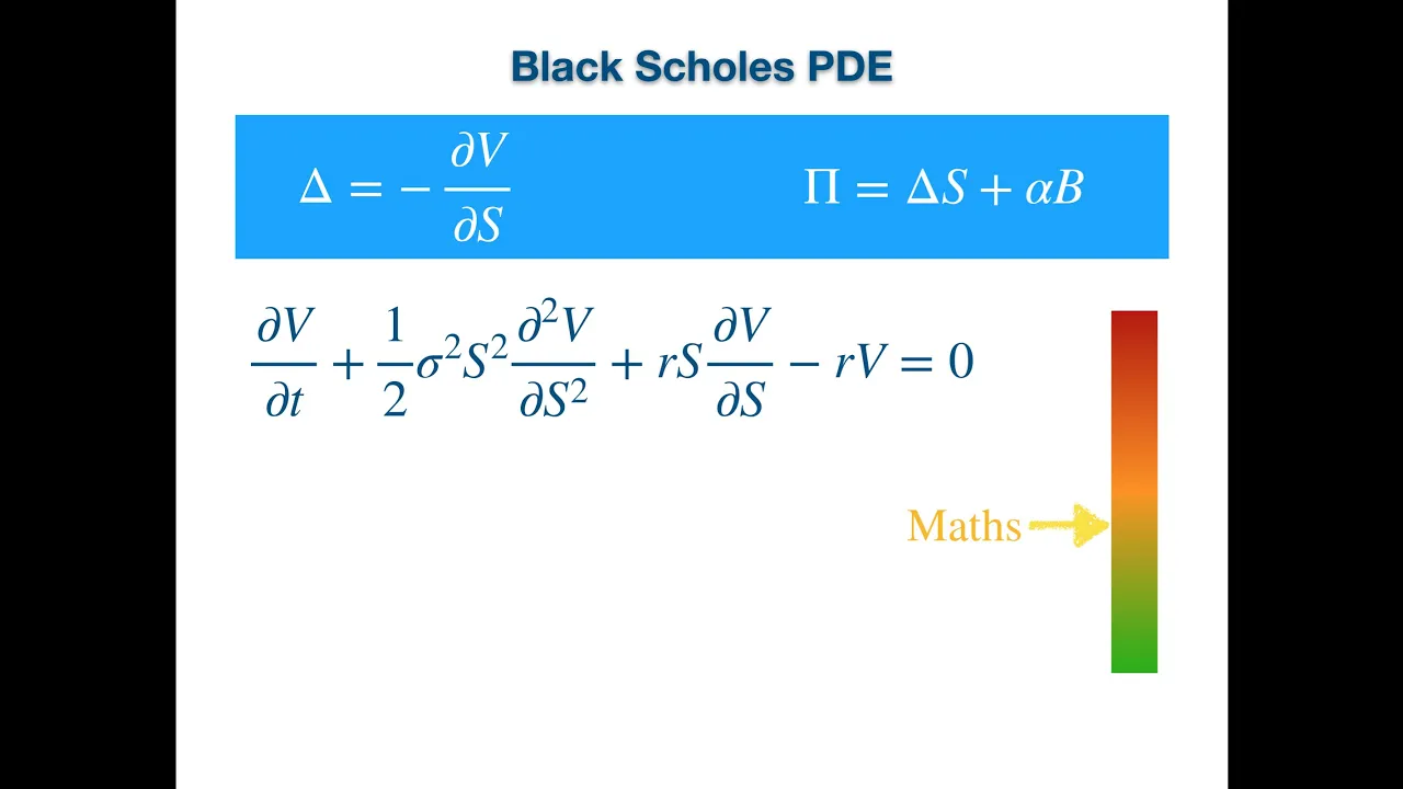
Black-Scholes PDE Derivation via Delta Hedging
@quantpie
41.3K views•2019-06-16

4:43
Elliptic Curve Cryptography Explained: ECC, ECDSA, ECDH
@PracticalNetworking
28.5K views•2024-10-21

10:44
Fourier Series Introduction: The Big Idea Explained
@DrTrefor
387K views•2021-05-03

6:00
The Mathematical Impossibility of Accurate World Maps
@Vox
23.3M views•2016-12-02
Related Study Plans & Knowledge Roadmaps
Structured learning paths in Mathematics
mathematics
Tensor Calculus: Vectors to Riemann Curvature
01Mathematical Foundations: Linear Algebra & Calculus
02Covectors, Dual Spaces, and Tensor Basics
03The Metric Tensor and Index Gymnastics
+ 2 more learning modules
40h5 modules
Explore Roadmap
mathematics
Gödel's Incompleteness: Logic, Proofs & Limits
01Introduction to Formal Systems & Hilbert's Dream
02Set Theory, Cardinality, and Cantor's Diagonal Argument
03Arithmetization and Gödel Numbering
+ 2 more learning modules
14h5 modules
Explore Roadmap
mathematics
Galois Theory: Fields, Groups & Solvability
01Foundations of Abstract Algebra: Groups & Fields
02Polynomials & Field Extensions
03Splitting Fields & Symmetries
+ 2 more learning modules
24h5 modules
Explore Roadmap
mathematics
Non-Euclidean Geometry: Models & Geodesics
01Euclid's Fifth Postulate and the Birth of New Geometries
02Hyperbolic Space and the Poincaré Disk Model
03Geodesics: Defining Straight Lines in Curved Spaces
+ 2 more learning modules
15h5 modules
Explore Roadmap